STCE Newsletter

1. The intensity of proton flares (13 Jan 2014 - 19 Jan 2014)
2. Review of solar activity (13 Jan 2014 - 19 Jan 2014)
3. Noticeable Solar Events (13 Jan 2014 - 19 Jan 2014)
4. Review of geomagnetic activity (13 Jan 2014 - 19 Jan 2014)
5. Geomagnetic Observations at Dourbes (13 Jan 2014 - 19 Jan 2014)
6. PROBA2 Observations (13 Jan 2014 - 19 Jan 2014)
7. Review of ionospheric activity (13 Jan 2014 - 19 Jan 2014)

The intensity of proton flares (13 Jan 2014 - 19 Jan 2014)

Solar activity seems to have shifted into higher gear. Indeed, 2014 has hardly started, yet we have already recorded 2 proton events (see previous STCE Newsletter at http://stce.be/news/232/welcome.html ). A proton is the positively charged nucleus of the hydrogen atom. For reasons solar scientists do not fully understand, these protons are sometimes released during (usually) strong solar flares. The particles travel at very high speeds (several 10.000 km/s!) and can bridge the Sun-Earth distance in a matter of hours. For example, during the Bastille Day event (14 July 2000), the first protons arrived already within 30 minutes after the peak of the solar flare (images underneath).

Because of their high speed, protons can have very high energies. As such, they constitute a radiation threat to astronauts, in particular during their extra-vehicular activities (space walks). They can increase the radiation dose of the crew and passengers on transpolar flights, and can cause communication problems over the polar areas (the so-called "Polar Cap Absorption"). These particles also give satellites a hard time. They can create malfunctions in the onboard electronic circuitry, degrade solar panel efficiency, and increase the noise in star-tracking systems. No wonder that space weather centers keep an eye on these malicious little creeps!

During the nineties, NOAA developed a scale to categorize the intensity of these events. This S-scale (http://www.swpc.noaa.gov/NOAAscales/index.html#SolarRadiationStorms ), short for solar radiation storm, has 5 levels going from minor (S=1) to extreme (S=5). In order to be categorized as a solar proton event (SPE), one looks at the number of protons having an energy of at least 10 MeV (a unit of energy - see note 1). If the intensity of these protons is at least 10 pfu (a unit of flux intensity - see note 2) at geosynchronous altitudes, then it is categorized as an S1-event.

The interesting part is that this scale is actually logarithmic. Indeed, in order to have a moderate proton event (S2), the proton flux needs to reach 100 pfu (=10*10), not 20! And for a major event (S3), a 1000 pfu (=10*10*10) is required. Analogous steps for a severe (S=4) and extreme (S=5) proton event.

To get an idea what these numbers mean, let's take a look at what SOHO's LASCO/C3 coronagraph (http://sohowww.nascom.nasa.gov/ ) experiences when it is bombarded by all these energetic protons. For a scale of S=1 to S=4, the figure above depicts how the coronagraph's field of view is affected. The increasing number of white dots and stripes are all impacts of protons on the camera's pixels. No wonder that during a severe event, a satellite's star tracker can no longer distinguish between true stars and impacts from the protons, and can thus become disoriented. A satellite can direct itself away from the Sun, such that sunlight no longer reaches the solar panels and thus depriving itself of the precious energy.

So far this solar cycle, the Sun has produced only four S3 events and zero S4 events. The strongest was the 7 March 2012 event when flux levels reached 6530 pfu. During the previous solar cycle, six S4 events were produced, the strongest reaching 31.700 pfu on 6 November 2001 following an X-class solar flare 2 days earlier (see the image above).

No S5-event has been recorded since measurements began in 1976, but one of the strongest SPE of the space age took place early August 1972. This was right in between the Apollo-16 and -17 missions which took place resp. in April and December of the same year. The event accounted for about 70% of the total 10 MeV fluence for the complete solar cycle (SC20)! Since this large event made such a dominant contribution to the total solar cycle fluence, some research scientists decided to separate it from the other events, and to class it as an anomalously large (AL) event, in contrast to the remaining ordinary events. It is commonly accepted that if an Apollo mission had flown during the August 1972 event, the astronauts would have received severe (and potentially lethal) doses of radiation (Note 3 for reference and further reading).

Note 1 - 10 MeV = 10 million eV. The eV (electron volt) is a very tiny amount of energy corresponding to about 0.16 billionth of a billionth of a Joule. For comparison, a flying mosquito has a kinetic energy of about a trillion eV (= 1000 billion eV).

Note 2 - pfu: proton flux unit. This is the number of particles registered per second, per square cm, and per steradian.

Note 3 - Further reading at SPENVIS (https://www.spenvis.oma.be/help/background/flare/flare.html ), ESA's SW web server (http://www.esa-spaceweather.net/spweather/BACKGROUND/EFFECTS/BIOLOGICAL/intro_biological.html ) and Science at NASA (http://www.nasa.gov/mission_pages/stereo/news/stereo_astronauts.html , http://science1.nasa.gov/science-news/science-at-nasa/2009/03jun_fakeastronaut/ and http://science1.nasa.gov/science-news/science-at-nasa/2005/27jan_solarflares/ ).

Review of solar activity (13 Jan 2014 - 19 Jan 2014)

One M-class flare and thirty C-class flares were reported by GOES during this week. The majority of flares occurred in NOAA AR 1959 at the moment the region was situated behind and close to the east solar limb.

The strongest flare of the week was the M1.3 flare on January 13, peaking at 21:51 UT. The flare originated from the Catania sunspot group 98 (NOAA AR 1944), the biggest and the most complex region observed this week and appears as a spike in the GOES X-ray curve: the flare started at 21:48UT and ended already at 21:53 UT.

Two partial halo CMEs were observed this week. A first plasma eruption took place during the first part of January 14 in the neighbourhood of Catania sunspot group 9 (NOAA AR 1950). It was accompanied by a coronal dimming, an EIT wave and a post-eruption arcade was observed by SDO/AIA.

The associated partial halo CME was first seen in the SOHO/LASCO C2 field of view at 09:24 UT. The CME had a width of about 180 degrees and approximate speed of 400 km/s. The bulk of the CME mass was directed northward of the Sun-Earth line. There was no signature in ACE data of a shock in the days after the lift-off.

The second partial halo CME this week, was first seen in the SOHO/LASCO C2 field of view at 23:24 UT on January 16. The CME was associated with the limb C6.2 flare which peaked at 21:39 UT on January 16.The CME had angular width of about 190 degrees, projected speed around 500 km/s and was directed somewhat southward of the Sun-Earth line. No shock arrival was detected by ACE as expected since this was a limb event.

A northern coronal hole reached the central meridian early on January 18.

Noticeable Solar Events (13 Jan 2014 - 19 Jan 2014)

DAY	BEGIN	MAX	END	LOC	XRAY	OP	10CM	TYPE	Cat	NOAA
13	2148	2151	2153		M1.3	F	94		98	1944

LOC: approximate heliographic location	TYPE: radio burst type
XRAY: X-ray flare class	Cat: Catania sunspot group number
OP: optical flare class	NOAA: NOAA active region number
10CM: peak 10 cm radio flux

Review of geomagnetic activity (13 Jan 2014 - 19 Jan 2014)

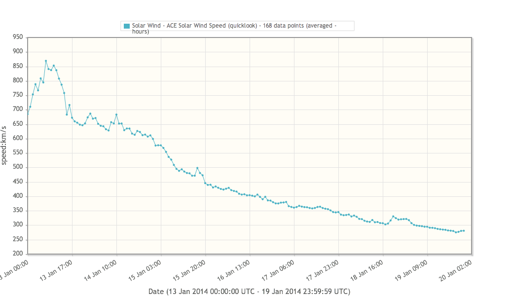
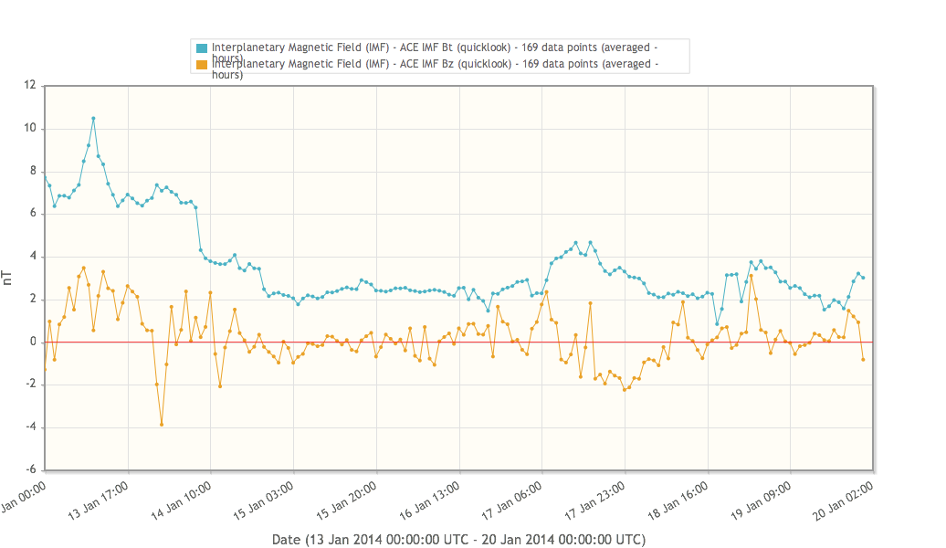
At first, the Earth was inside a fast solar wind associated with the extended (in latitude and in longitude) coronal hole in the northern hemisphere which first reached the central meridian on January 8. The solar wind speed reached a maximum value of about 870 km/s on January 13. The interplanetary magnetic field reached a maximum value of about 10 nT on that day. The interaction region between the slow and fast solar wind and the actual high speed stream emanating from the coronal hole high speed stream did not result in disturbed geomagnetic condition.

During the rest of the week, the interplanetary magnetic field was stable between 2 and 3 nT.

NOAA reported quiet geomagnetic conditions for the whole week except for a few intervals of Kp = 3.

Geomagnetic Observations at Dourbes (13 Jan 2014 - 19 Jan 2014)

PROBA2 Observations (13 Jan 2014 - 19 Jan 2014)

Solar Activity
Solar flare activity fluctuated between low and moderate during the week.
In order to view the activity of this week in more detail, we suggest to go to the following website from which all the daily (normal and difference) movies can be accessed: http://proba2.oma.be/ssa
This page also lists the recorded flaring events.
A weekly overview movie can be found here (SWAP week 199).
http://proba2.oma.be/swap/data/mpg/movies/WeeklyReportMovies/WR199_Jan13_Jan19/weekly_movie_2014_01_13.mp4

Details about some of this week's events, can be found further below.

Monday Jan 13:

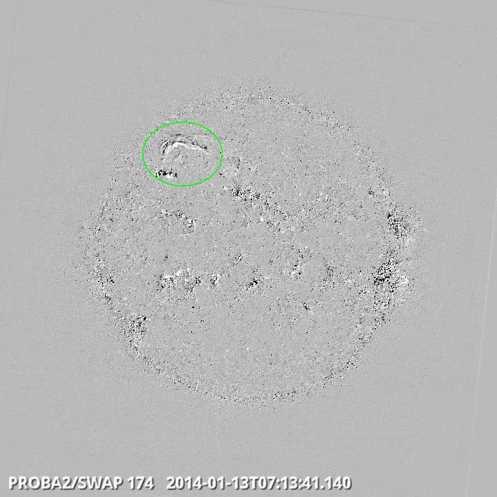
Eruption in the north east quadrant @ 07:13 ­ SWAP difference image
Find a movie of the events here (SWAP difference movie)
http://proba2.oma.be/swap/data/mpg/movies/WeeklyReportMovies/WR199_Jan13_Jan19/Events/20140113_Eruption_NoertEastQuad_0713_swap_diff.mp4
Find a movie of the events here (SWAP movie)
http://proba2.oma.be/swap/data/mpg/movies/WeeklyReportMovies/WR199_Jan13_Jan19/Events/20140113_Eruption_NoertEastQuad_0713_swap_movie.mp4

Wednesday Jan 15:

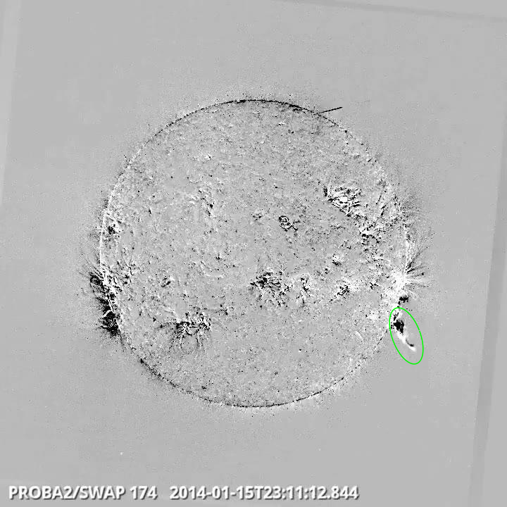
Eruption on the west limb @ 23:11 ­ SWAP difference image
Find a movie of the event here (SWAP difference movie)
http://proba2.oma.be/swap/data/mpg/movies/WeeklyReportMovies/WR199_Jan13_Jan19/Events/20140115_Eruption_WestLimb_2311_swap_diff.mp4

Thursday Jan 16:

Friday Jan 17:

Eruption on the west limb @ 12:47 ­ SWAP difference image
Find a movie of the event here (SWAP difference movie)
http://proba2.oma.be/swap/data/mpg/movies/WeeklyReportMovies/WR199_Jan13_Jan19/Events/20140116_Eruption_WestLimb_1247_swap_diff.mp4
Find a movie of the event here (SWAP movie)
http://proba2.oma.be/swap/data/mpg/movies/WeeklyReportMovies/WR199_Jan13_Jan19/Events/20140116_Eruption_WestLimb_1247_swap_movie.mp4

Eruption on the east limb @ 15:33 ­ SWAP difference image
Find a movie of the event here (SWAP difference movie)
http://proba2.oma.be/swap/data/mpg/movies/WeeklyReportMovies/WR199_Jan13_Jan19/Events/20140117_Eruption_EastLimb_1533_swap_diff.mp4

Review of ionospheric activity (13 Jan 2014 - 19 Jan 2014)

The figure shows the time evolution of the Vertical Total Electron Content (VTEC) (in red) during the last week at three locations:
a) in the northern part of Europe(N61°, 5°E)
b) above Brussels(N50.5°, 4.5°E)
c) in the southern part of Europe(N36°, 5°E)
This figure also shows (in grey) the normal ionospheric behaviour expected based on the median VTEC from the 15 previous days.

The VTEC is expressed in TECu (with TECu=10^16 electrons per square meter) and is directly related to the signal propagation delay due to the ionosphere (in figure: delay on GPS L1 frequency).
The Sun's radiation ionizes the Earth's upper atmosphere, the ionosphere, located from about 60km to 1000km above the Earth's surface.The ionization process in the ionosphere produces ions and free electrons. These electrons perturb the propagation of the GNSS (Global Navigation Satellite System) signals by inducing a so-called ionospheric delay.

See http://stce.be/newsletter/GNSS_final.pdf for some more explanations ; for detailed information, see http://gnss.be/ionosphere_tutorial.php