
Contents
Sunspot group classification
The McIntosh classification for sunspot groups was developed by Patrick McIntosh (McIntosh, 1990) based on an earlier scheme devised by Max Waldmeier in 1947, called the Zürich classification (Carrasco et al. 2015). The general form of the McIntosh classification is Zpc (overview), where Z is the modified Zurich class, p is the type of principal spot, primarily describing the penumbra, and c is the degree of compactness in the interior of the group.
Z: Modified Zurich Class
The modified Zurich classes are defined on the basis of whether penumbra is present, how penumbra is distributed, and by the length of the group. Length is defined in absolute heliographic degrees. An unipolar group is a single spot, or a compact cluster of spots with the greatest separation between spots 3°. In the case of a group with penumbra (class H), the greatest separation is measured between the center of the attendant umbra and the nearest border of penumbra surrounding the main spot. A bipolar group has two or more spots forming an elongated cluster with a length of more than 3°. Usually there will be a space near the middle of the cluster dividing it into two distinct parts. Groups with a large principal spot must be 5° in length (i.e., 2.5° plus 3°) to be classified as bipolar.
A - unipolar group with no penumbra, representing either the formative or final stage of evolution in a sunspot group.
B - bipolar group without penumbra on any spots.
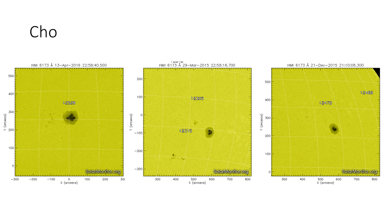
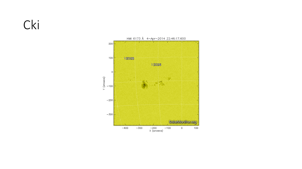
C - bipolar group with penumbra on one end of the group, in most cases surrounding the largest of the leader umbrae.
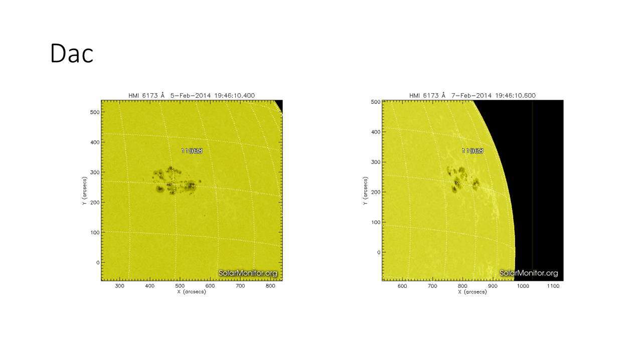
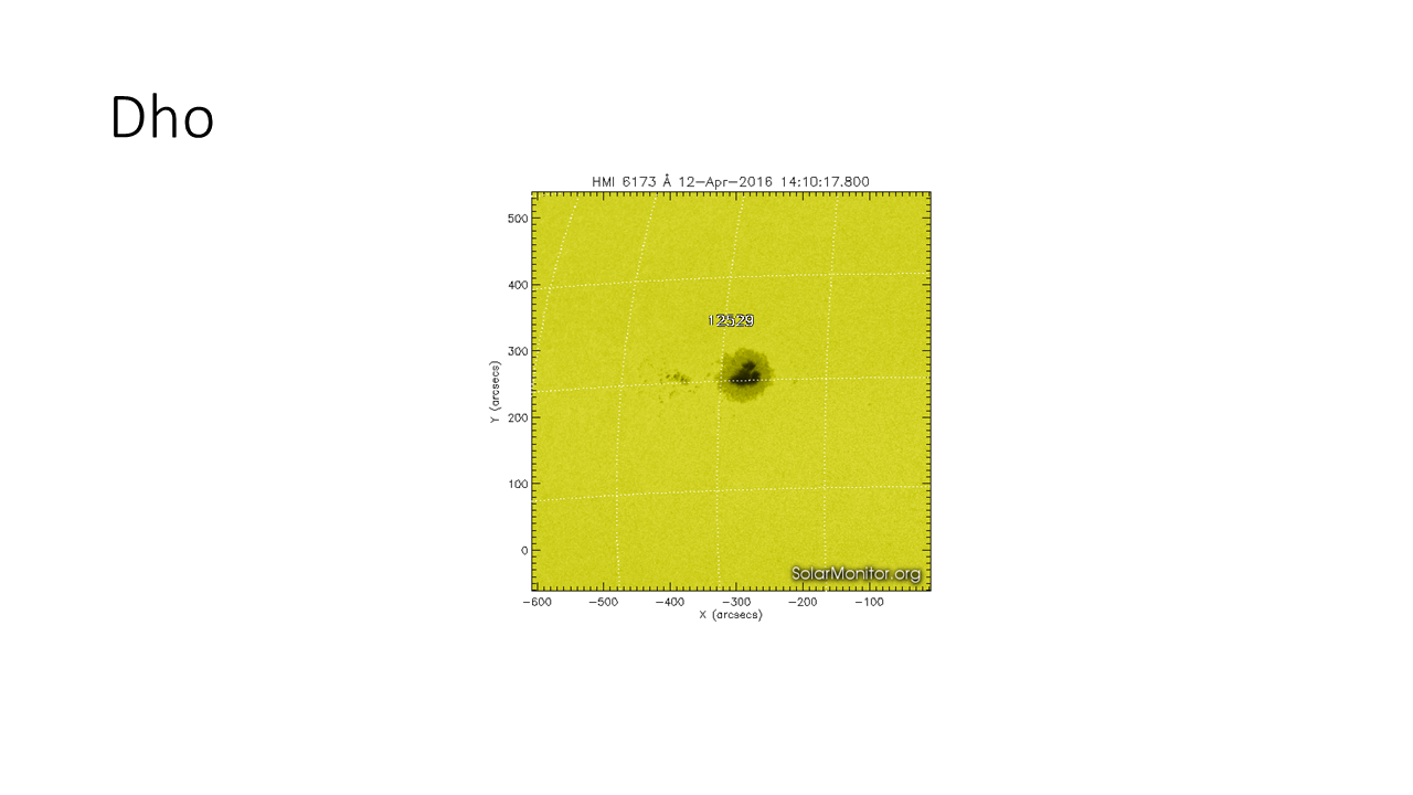
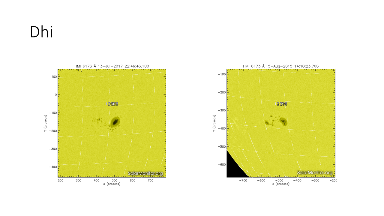
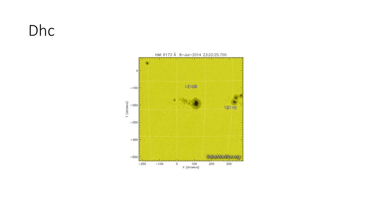
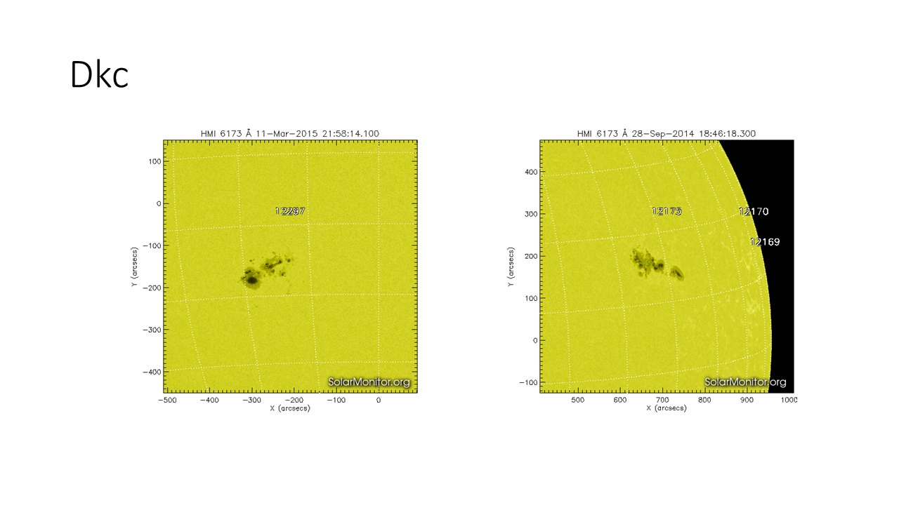
D - bipolar group with penumbra on spots at both ends of the group, and with length < 10°.
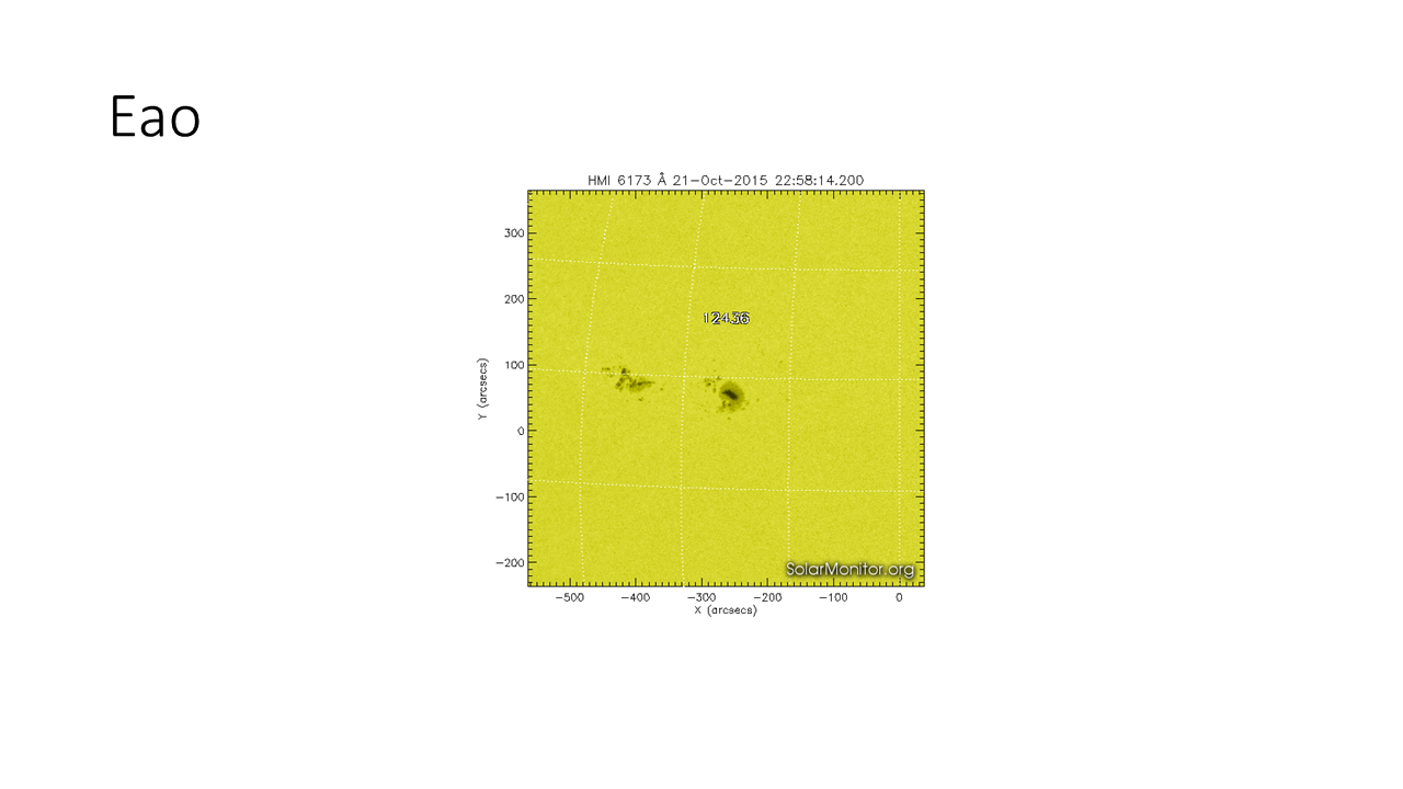
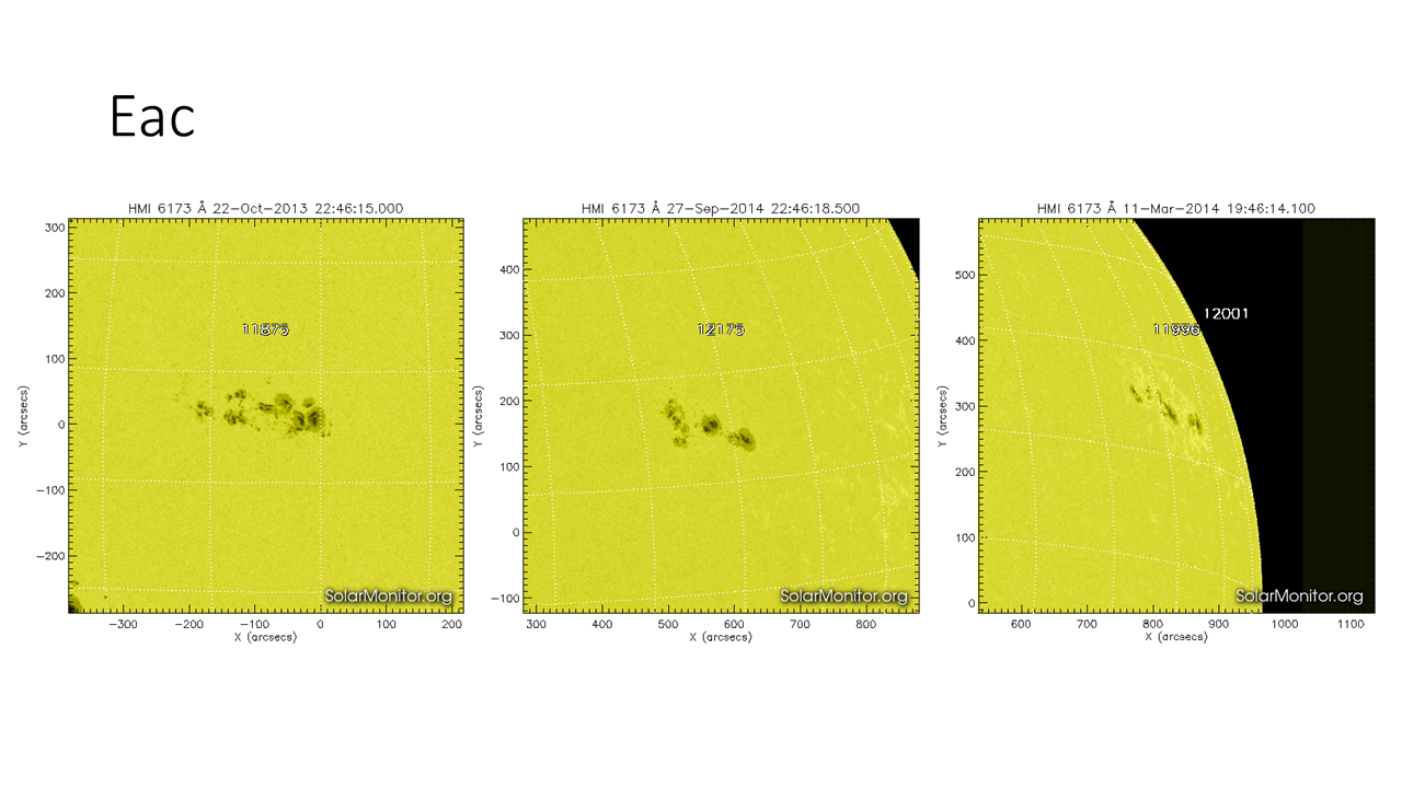
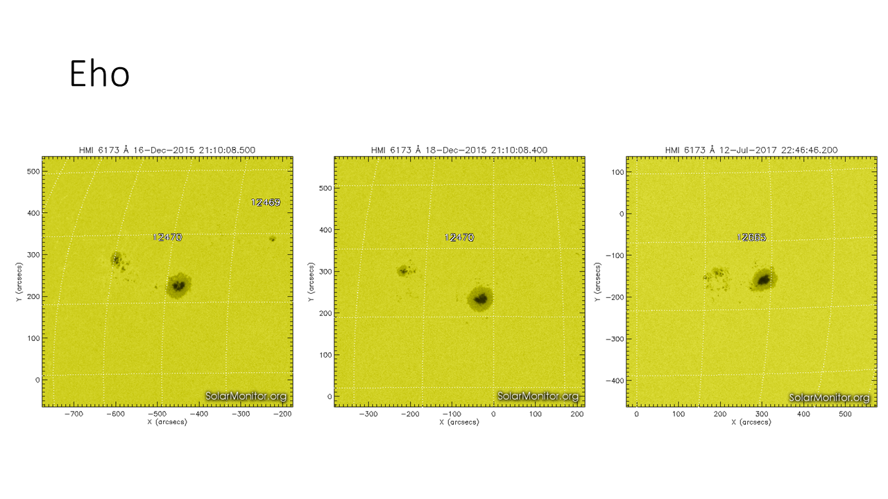
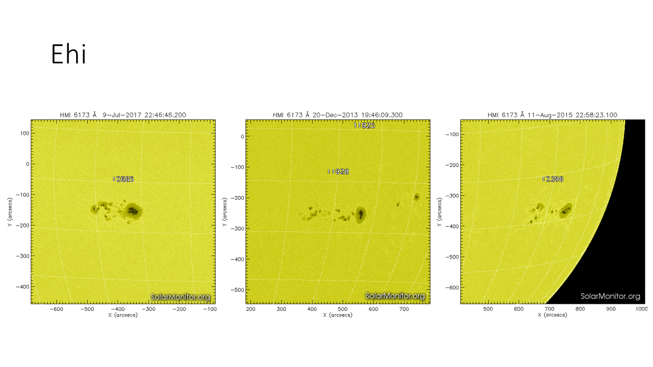
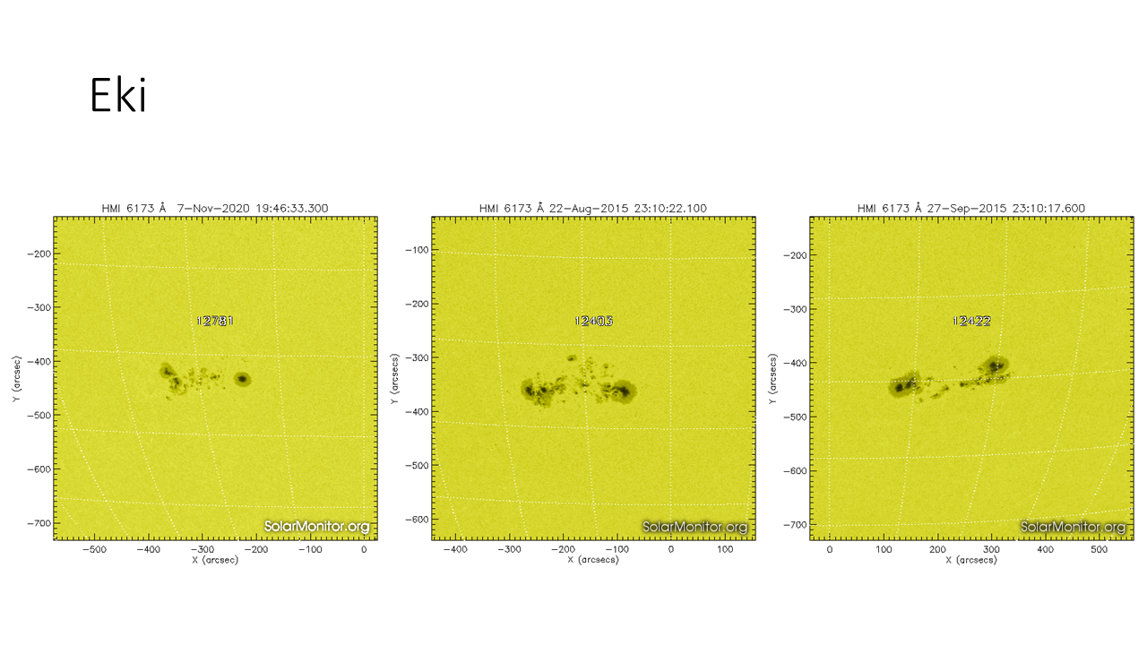
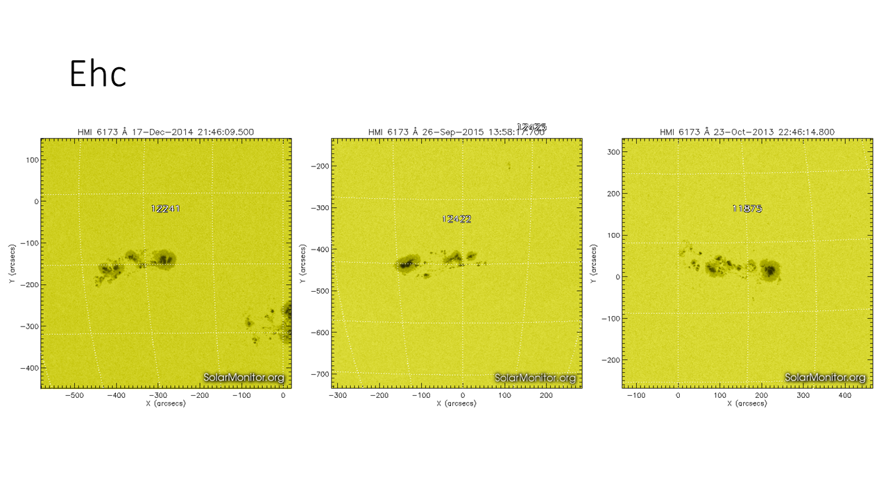
E - bipolar group with penumbra on spots at both ends of the group, and with length defined as: 10° < length < 15°.
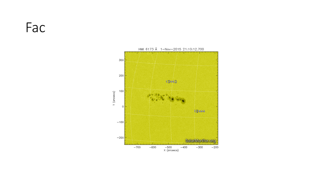
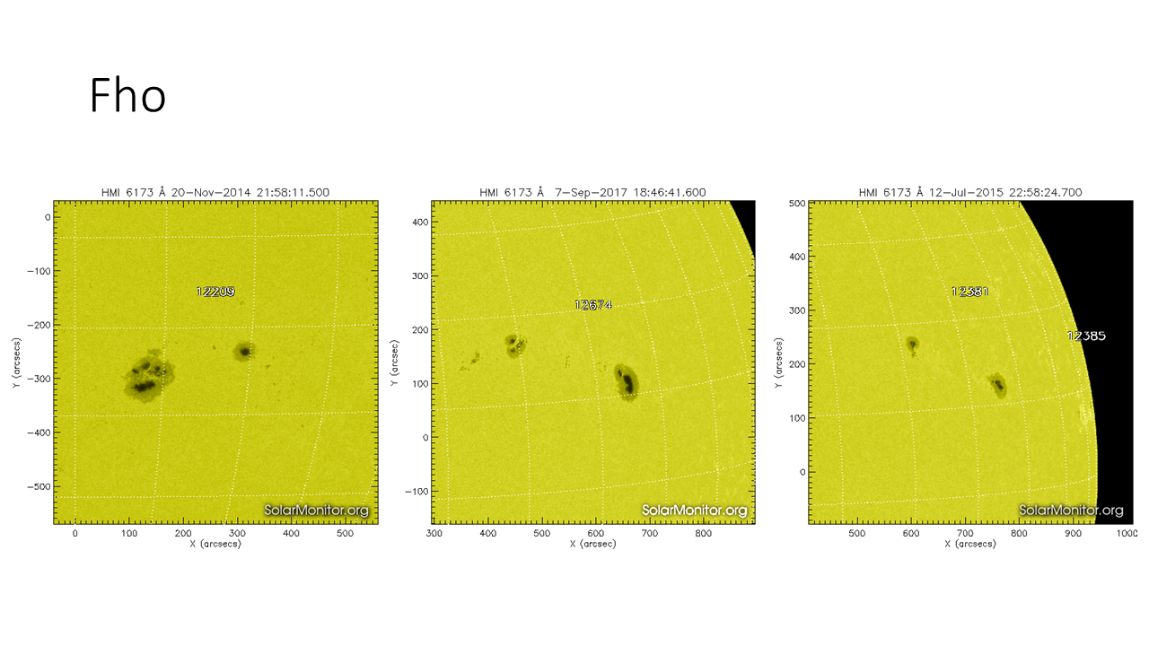
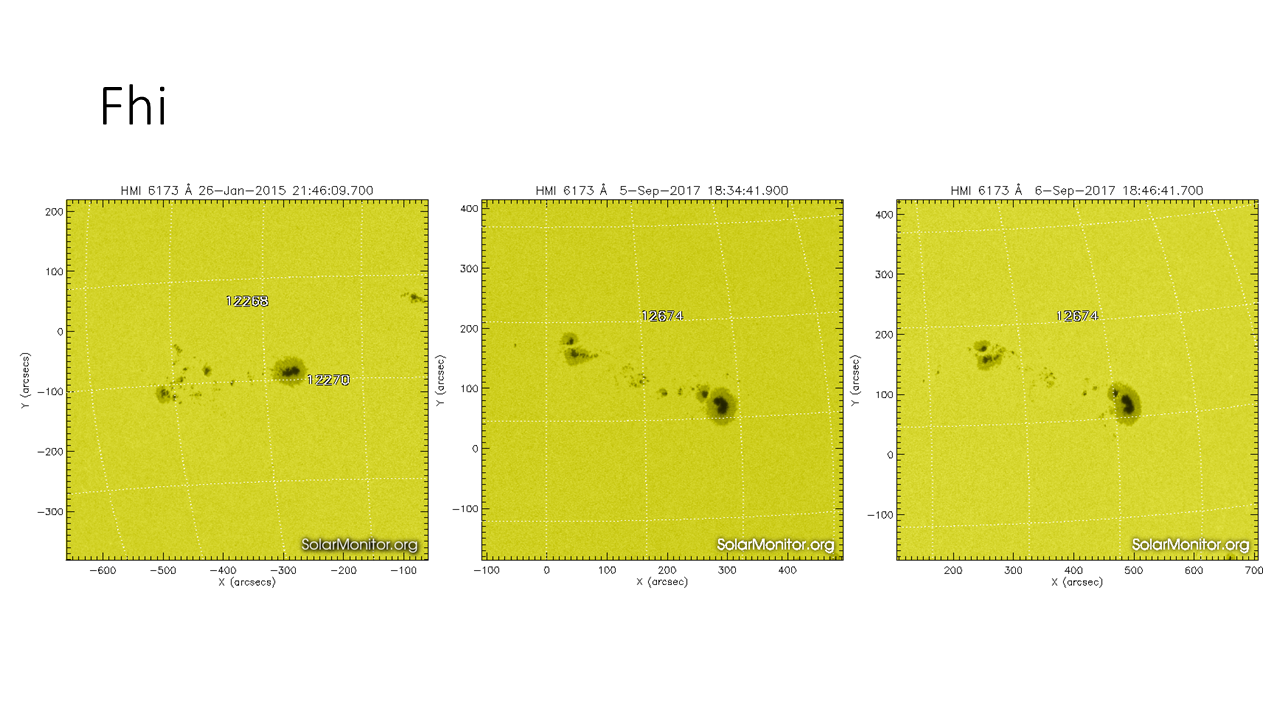
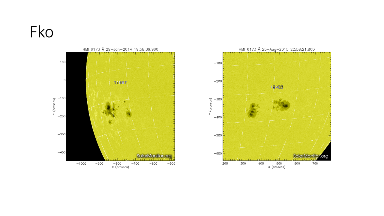
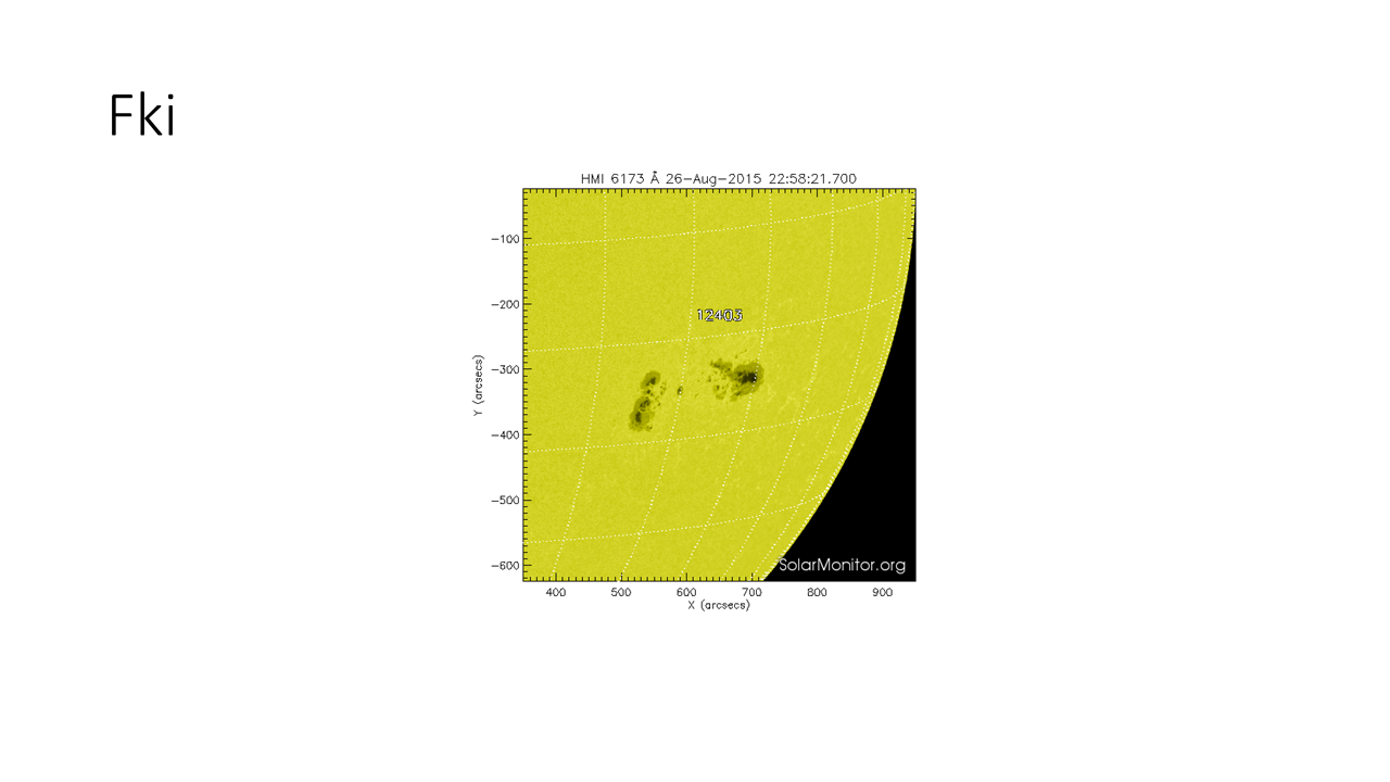
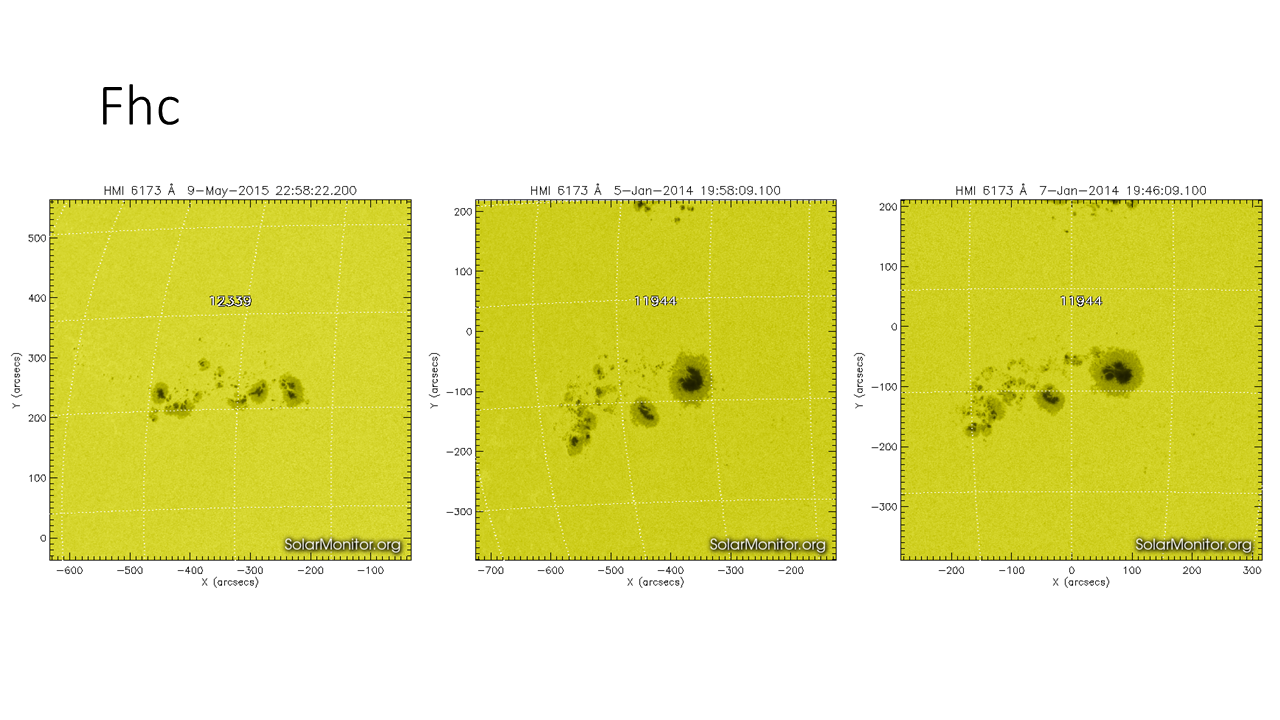
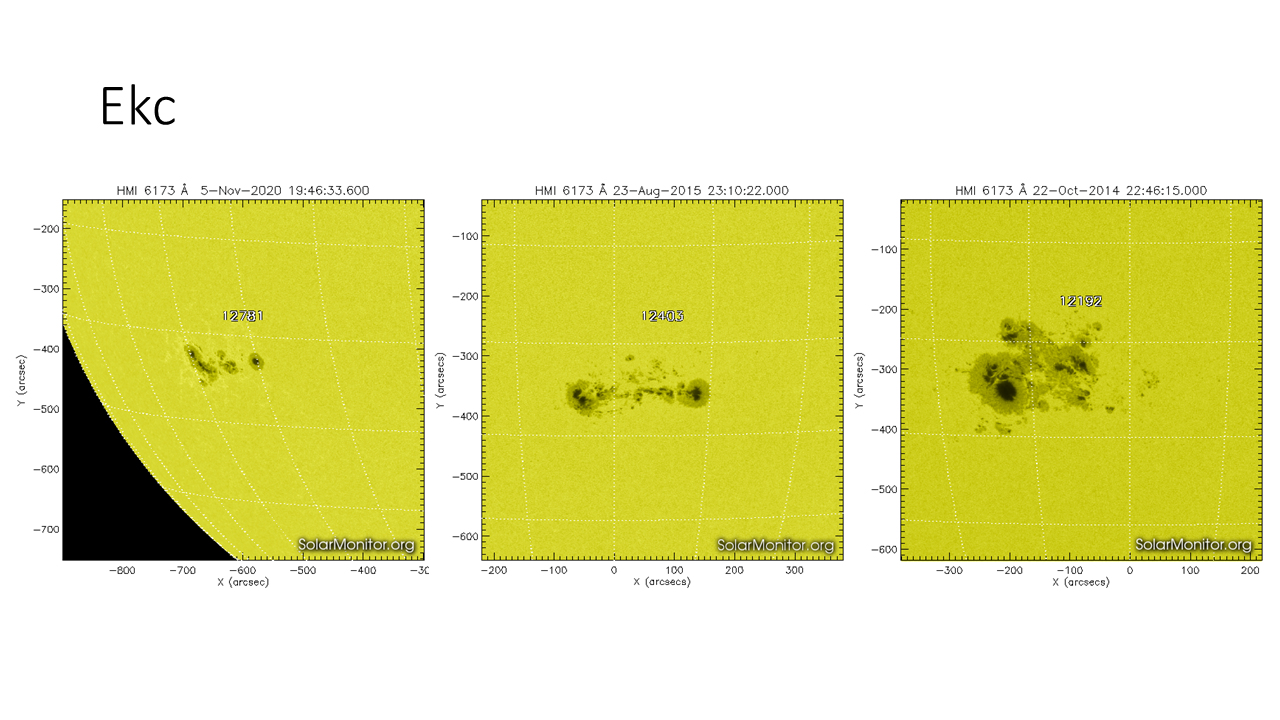
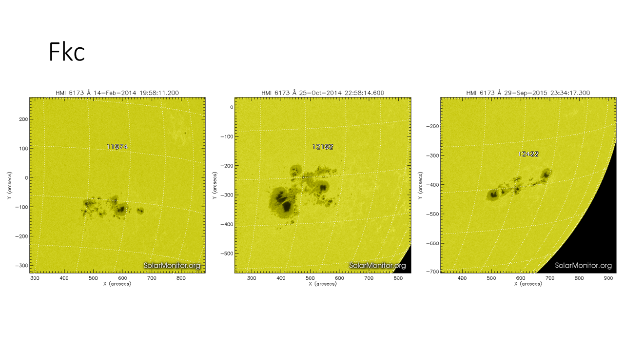
F - bipolar group with penumbra on spots at both ends of the group, and length > 15 °.
H - unipolar group with penumbra. The principal spot is usually the leader spot remaining from a pre-existing bipolar group.
p: Penumbra of the largest sunspot
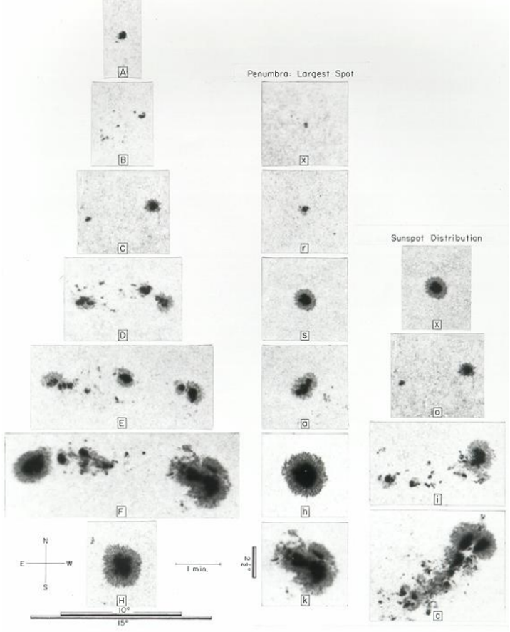
The type of largest spot in a sunspot group can be described by the combination of type of penumbra, size of penumbra, and symmetry of penumbra and umbrae within that penumbra.
x - no penumbra (group is class A or B).
r - rudimentary penumbra partially surrounds the largest spot. This penumbra is incomplete, granular rather than filamentary, brighter than mature penumbra, and extends as little as 3" from the spot umbra. Rudimentary penumbra may be either in a stage of formation or dissolution.
s - small, symmetric. Largest spot has mature, dark, filamentary penumbra of circular or elliptical shape with some irregularity along the border allowed. There is either a single umbra, or a compact cluster of umbrae, mimicking the symmetry of the penumbra. The north-south diameter across the penumbra is < 2.5°.
a - small, asymmetric. Penumbra of the largest spot is irregular in outline and the multiple umbrae within it are separated, not mimicking the symmetry of the penumbra. The north-south diameter of the penumbra is < 2.5°.
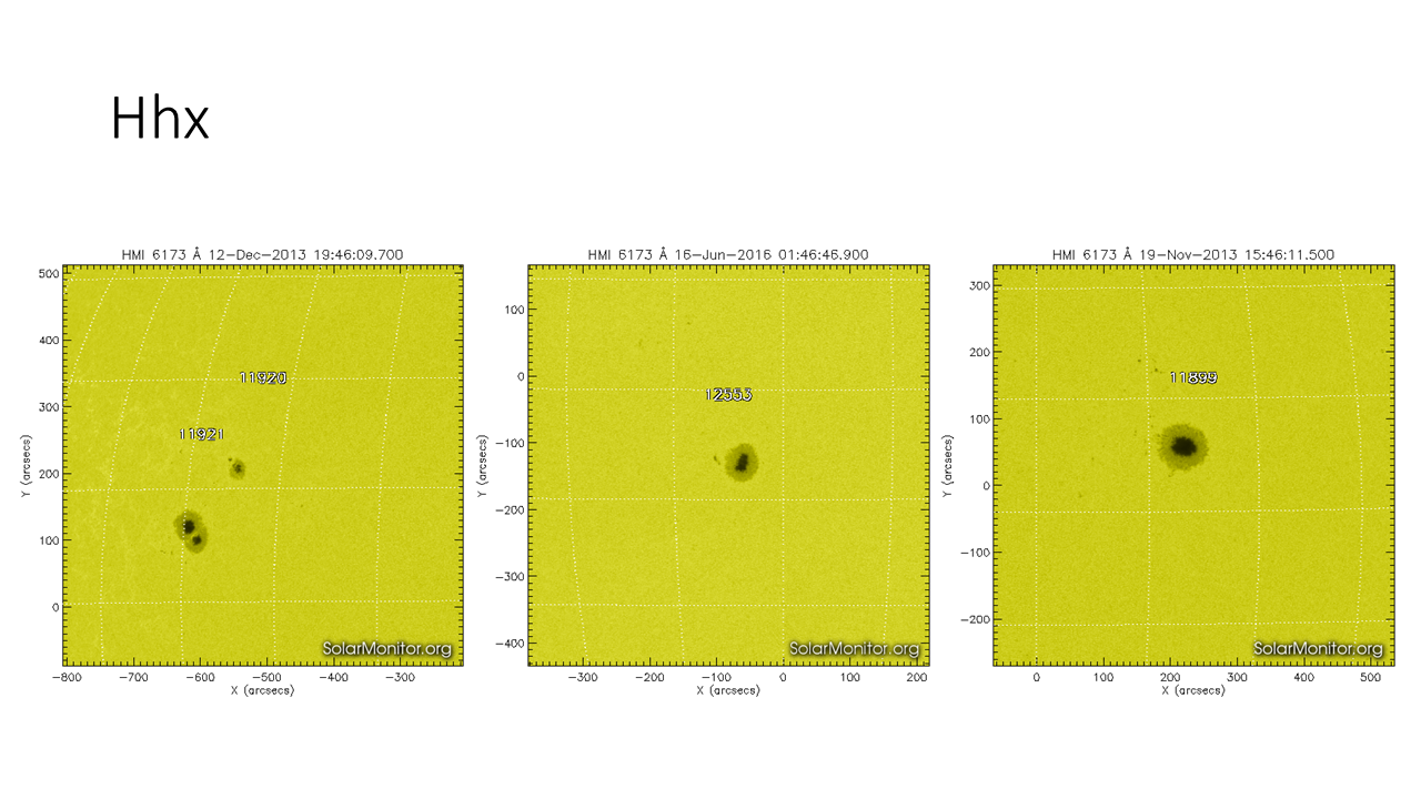
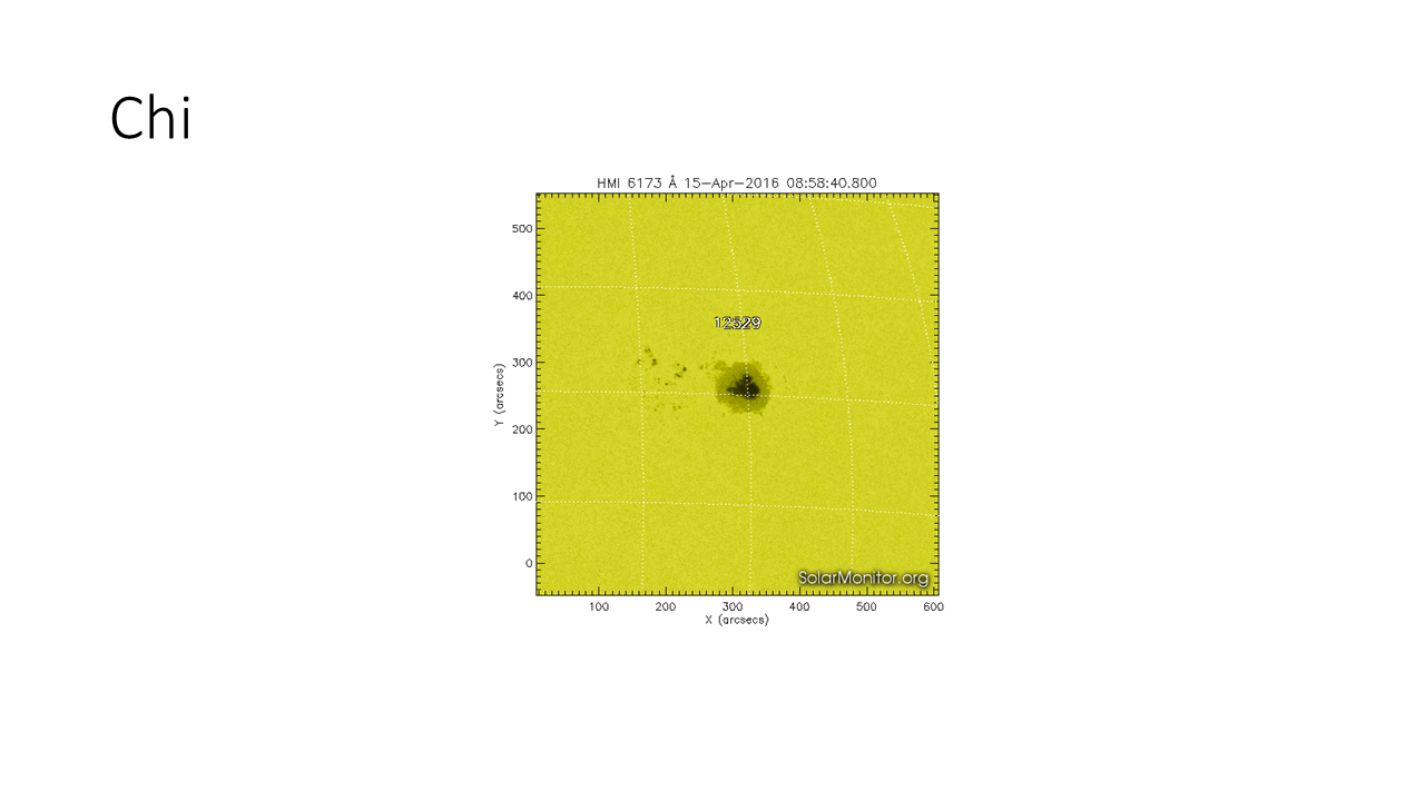
h - large, symmetric. Same structure as type 's', but the north-south diameter of the penumbra > 2.5°. Therefore, the area must be > 250 millionths of a solar hemisphere.
k - large, asymmetric. Same structure as type 'a', but the north-south diameter > 2.5°, and so the area > 250 millionths of a solar hemisphere.
c: Sunspot distribution
A simple ranking of the relative spottedness in the interior of a sunspot group gives additional information about the area of the group and, more important, whether there could be strong spots near the line of polarity inversion lying between the principal leader and follower spots.
x - undefined for unipolar groups (class A and H).
o - open. Few, if any, spots between leader and follower. Interior spots are of very small size.
i - intermediate. Numerous spots lie between the leading and following portions of the group, but none of them possesses a mature penumbra.
c - compact. The area between the leading and following ends of the spot group is populated with many strong spots, with at least one interior spot possessing mature penumbra. The extreme case of compact distribution has the entire spot group enveloped in one continuous penumbral area.
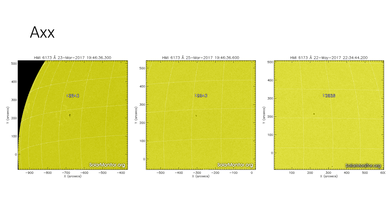
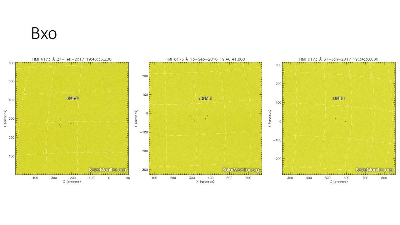
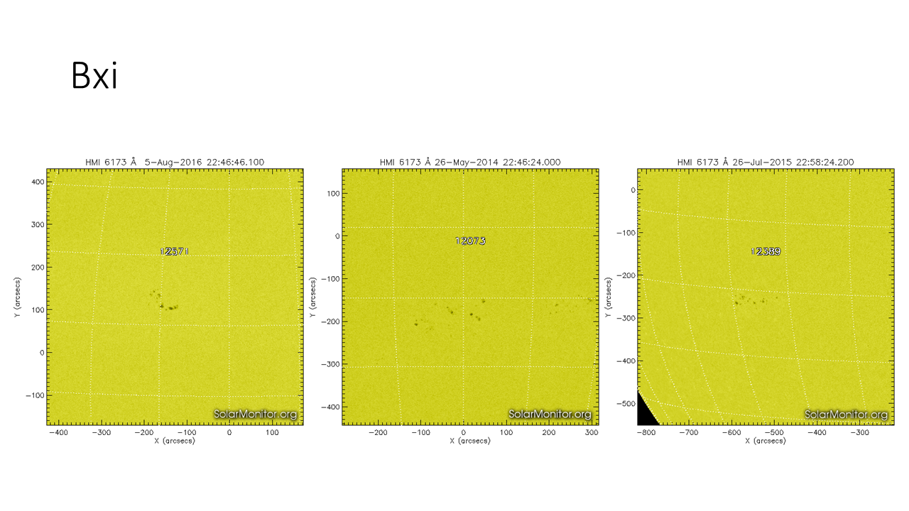
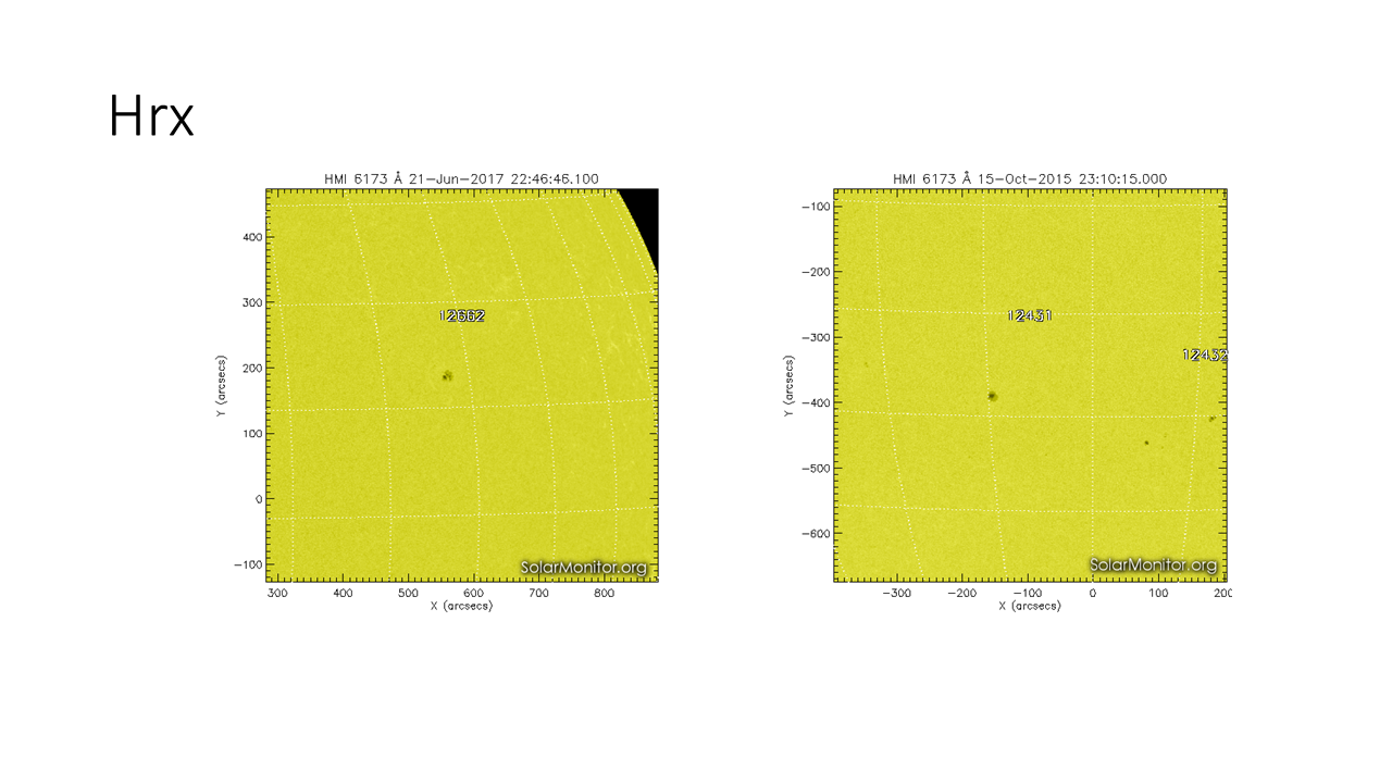
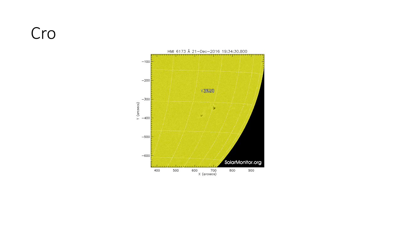
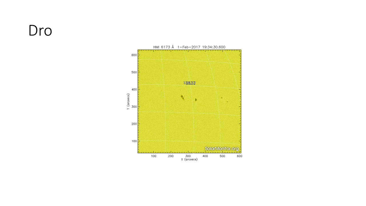
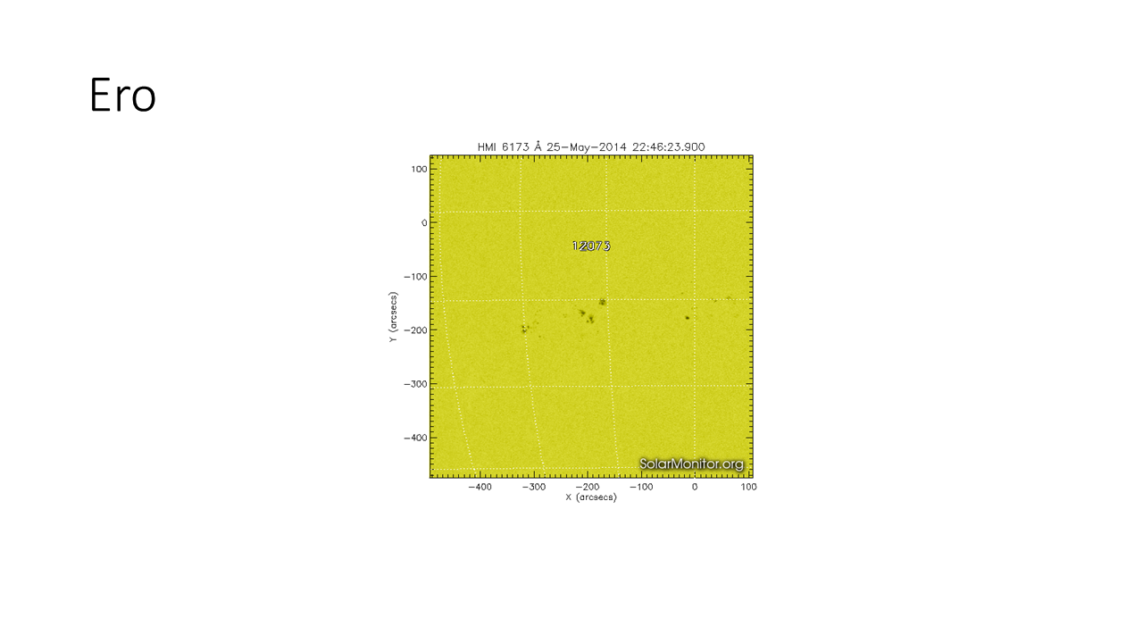
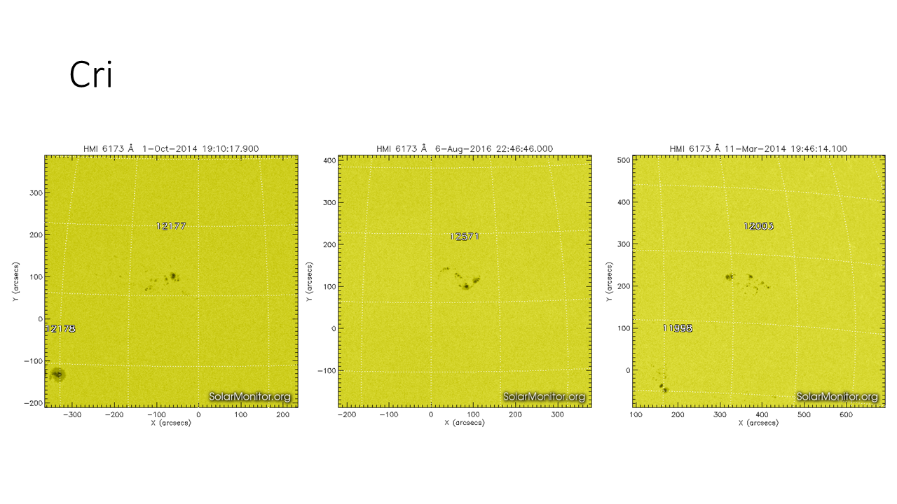
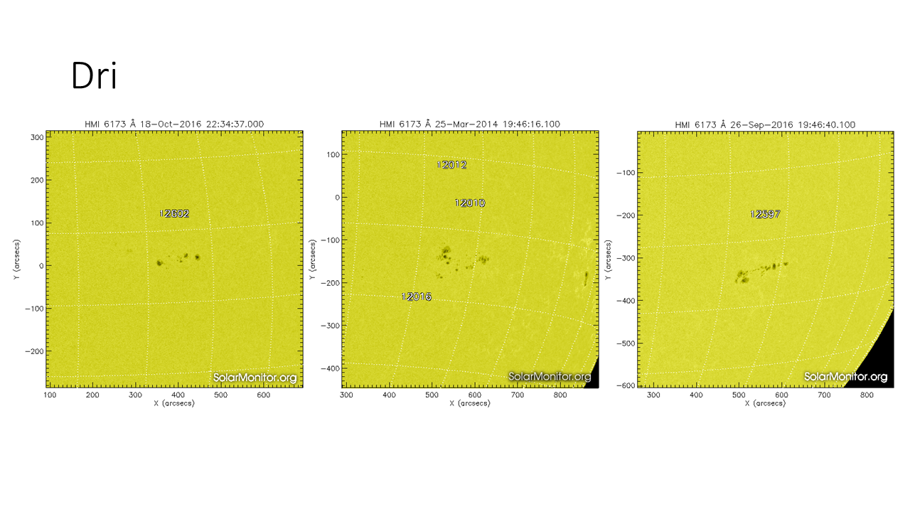
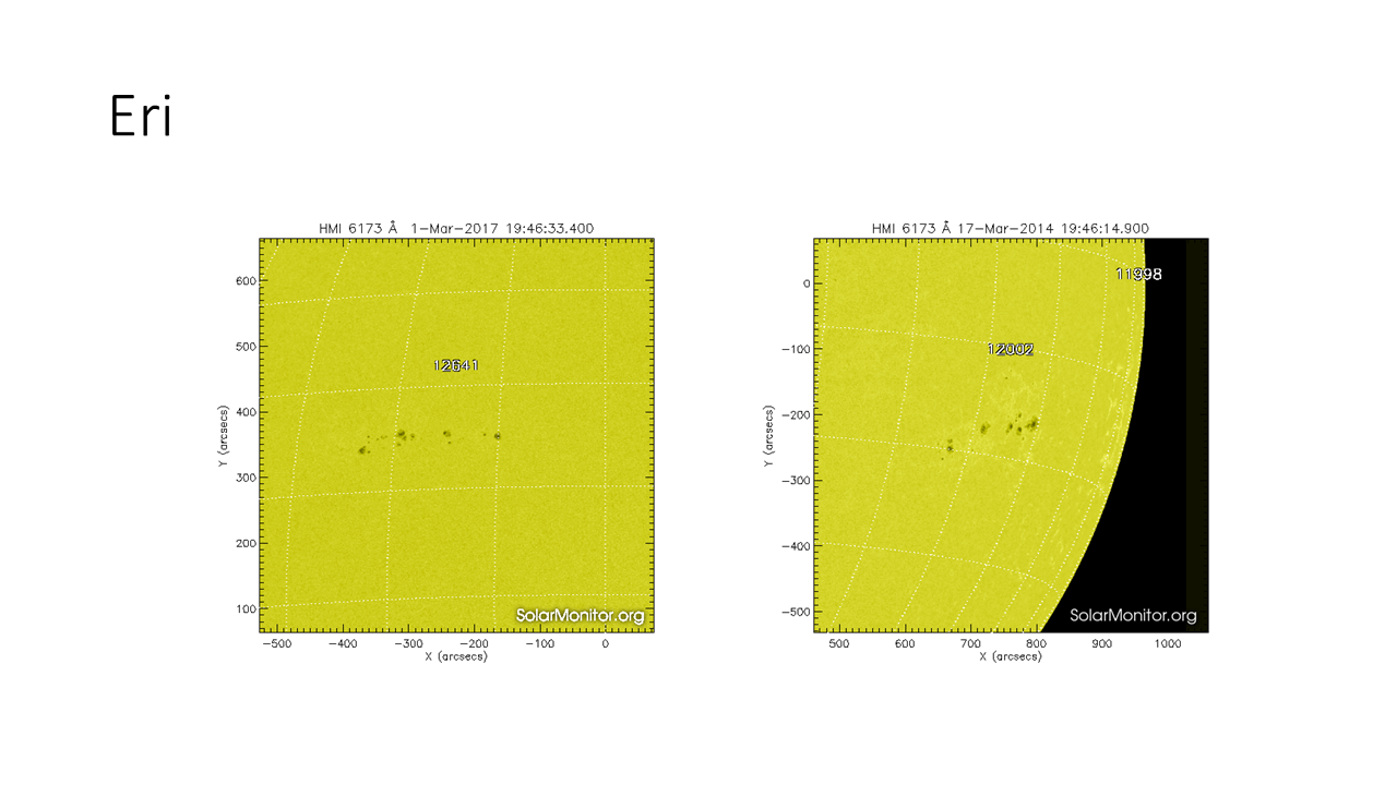
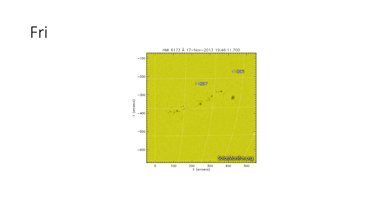
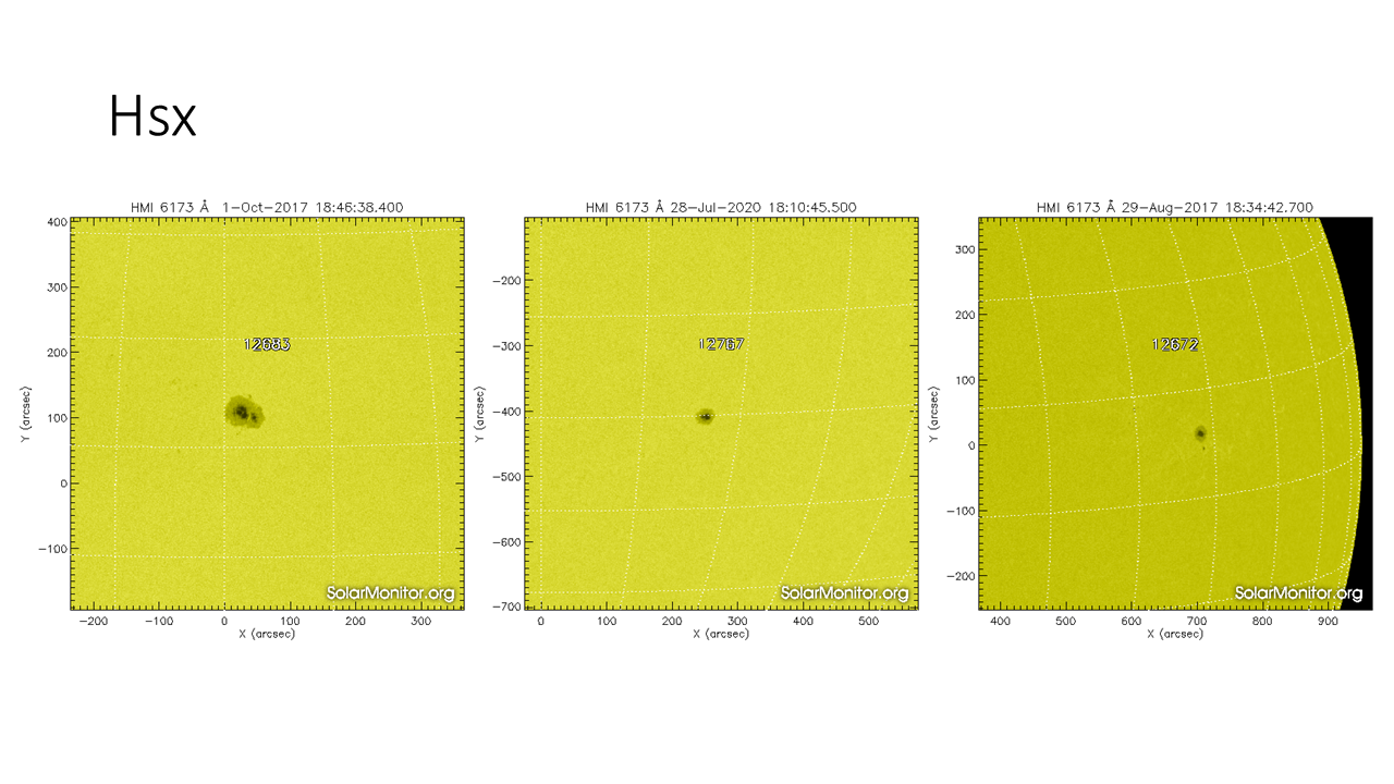
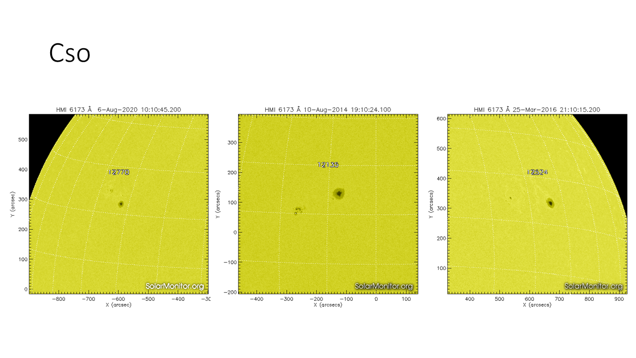
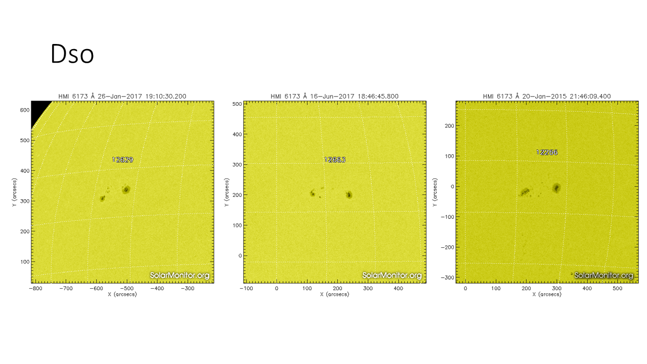
This three-component system leads to 60 valid classes, captured by table underneath and providing links to examples (the grids have a size of 10°x10°; courtesy SolarMonitor.org). The classes have been ordered with the smallest and simplest types in the upper-left portion of the table, and the largest and most complex sunspot groups in the lower-right portion. The McIntosh classification is a cornerstone in the prediction of the likelihood a flare of a certain intensity could be produced by a sunspot group of a certain McIntosh class. See e.g. Table 2 in Bloomfield et al. (2012).
| Axx | |||||
| Bxo | |||||
| Bxi | |||||
| Hrx | Cro | Dro | Ero | Fro | |
| Cri | Dri | Eri | Fri | ||
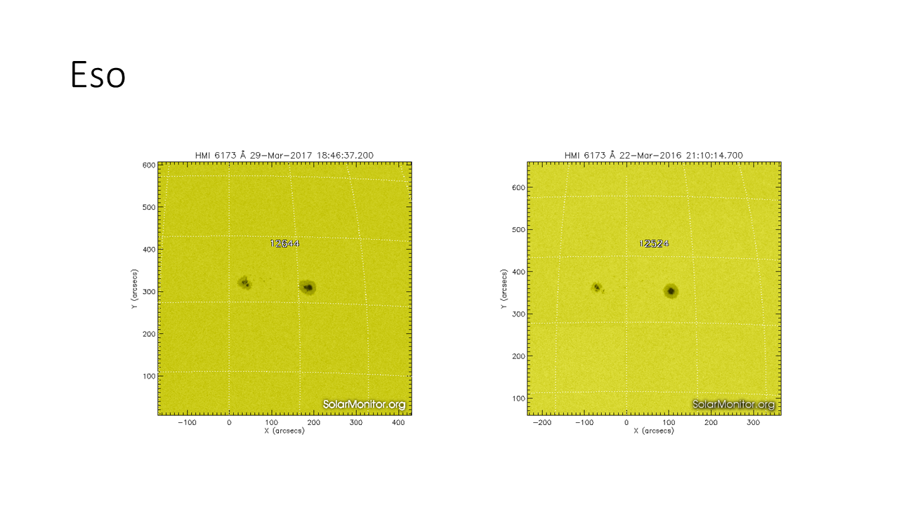
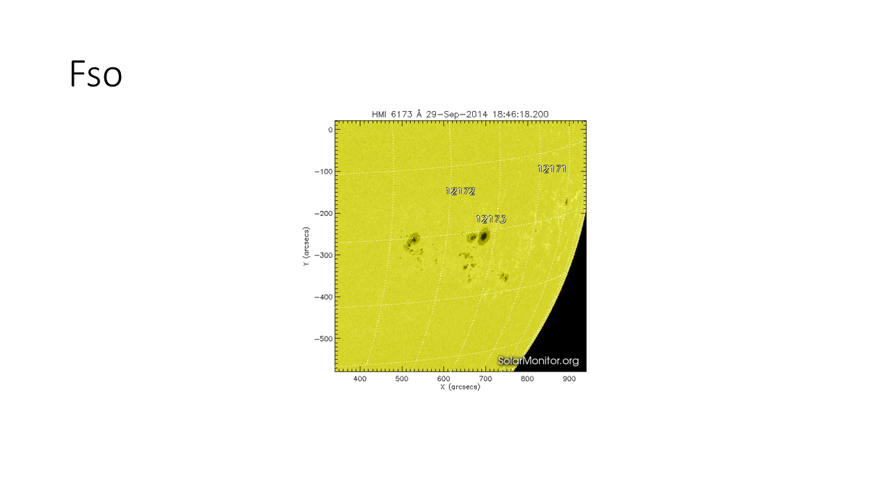
| Hsx | Cso | Dso | Eso | Fso | |
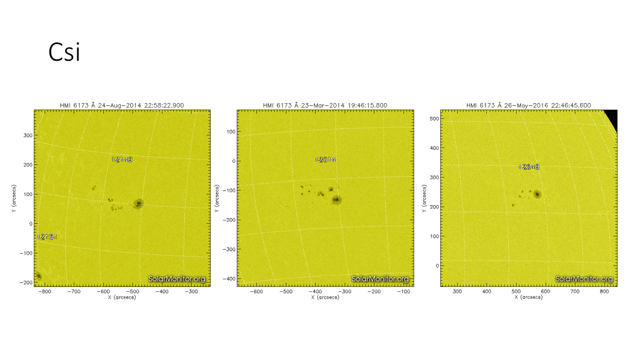
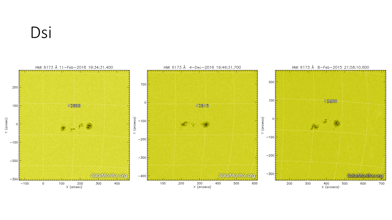
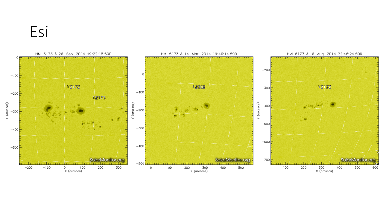
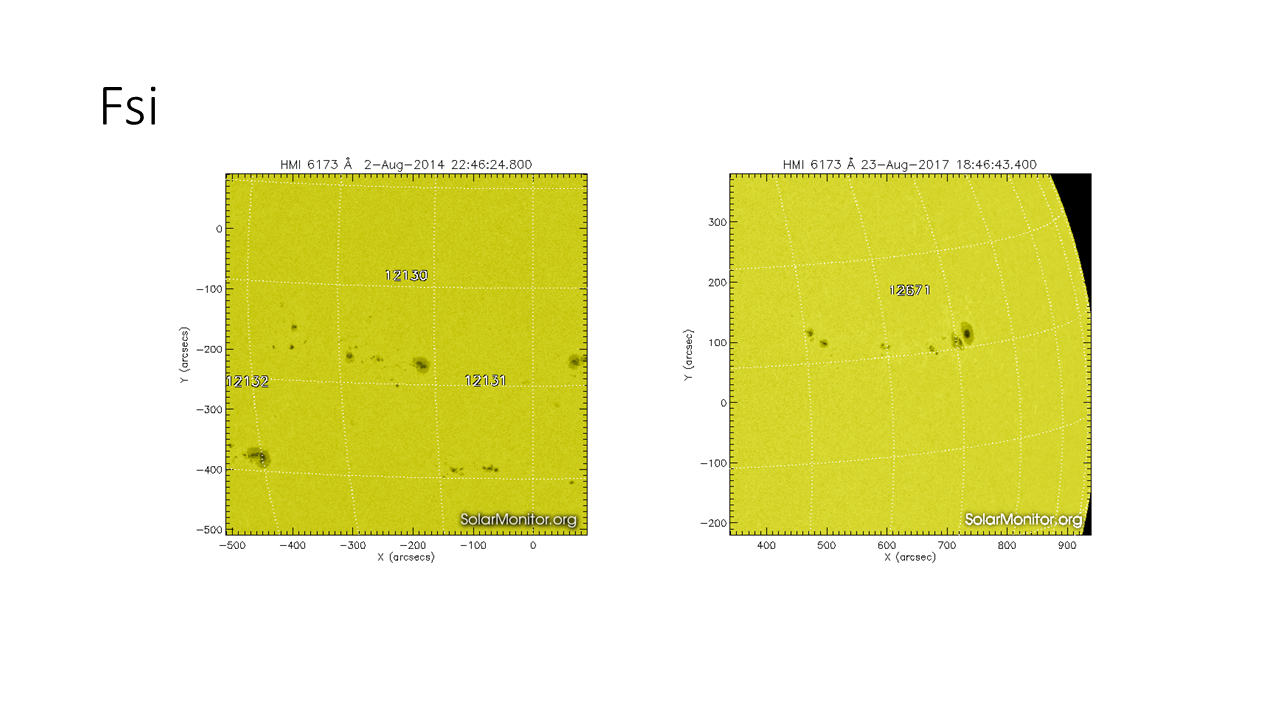
| Csi | Dsi | Esi | Fsi | ||
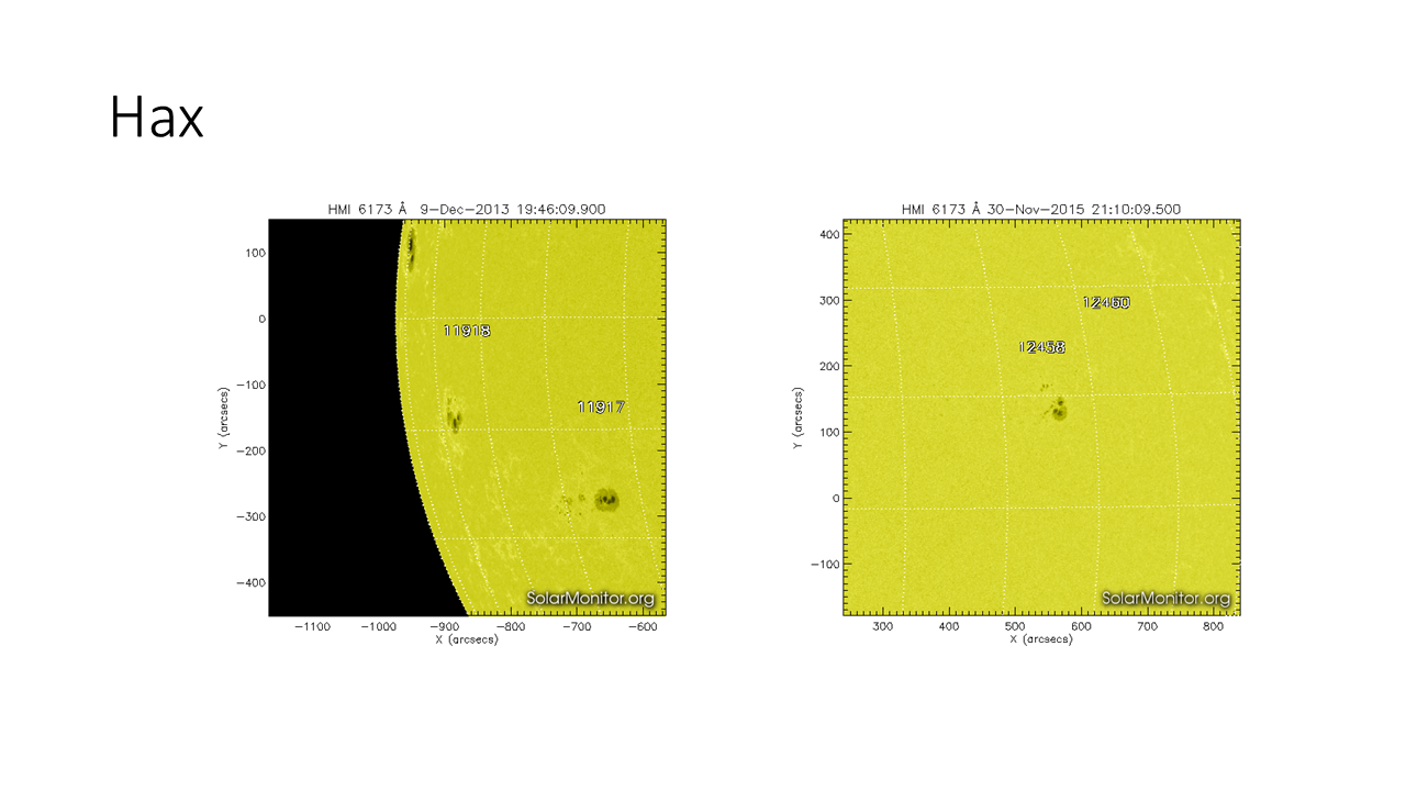
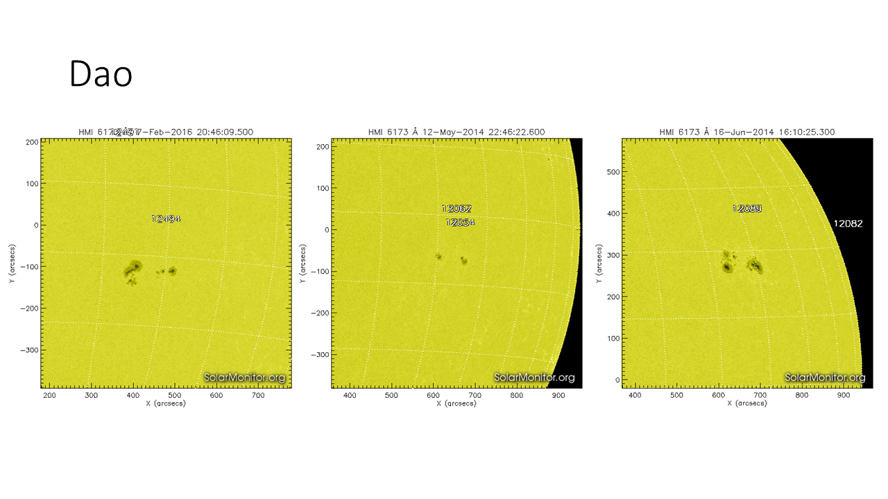
| Hax | Cao | Dao | Eao | Fao | |
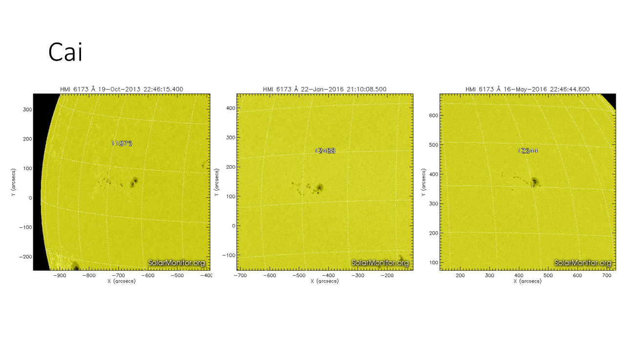
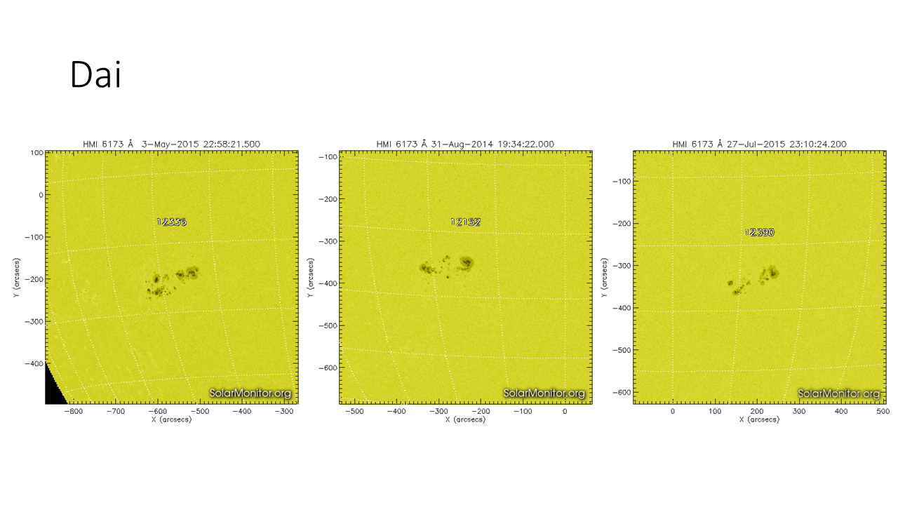
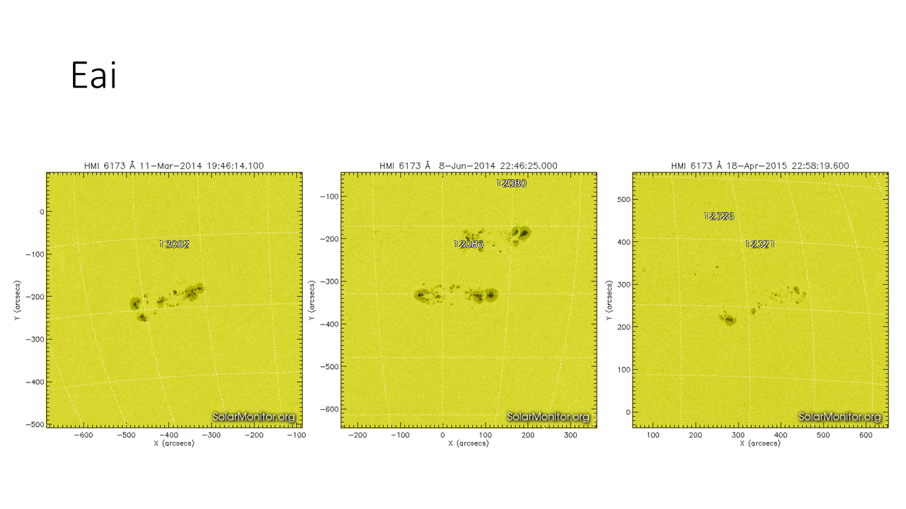
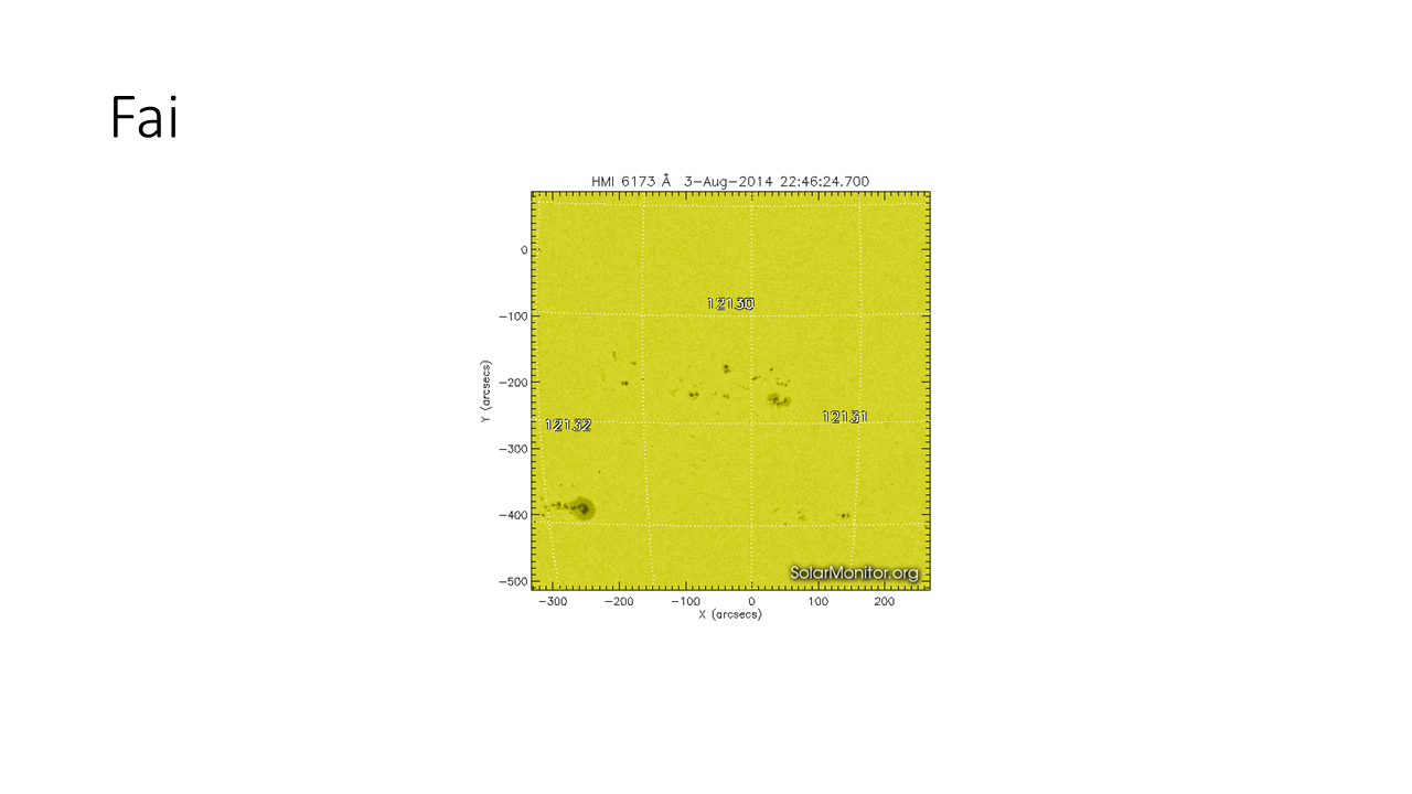
| Cai | Dai | Eai | Fai | ||
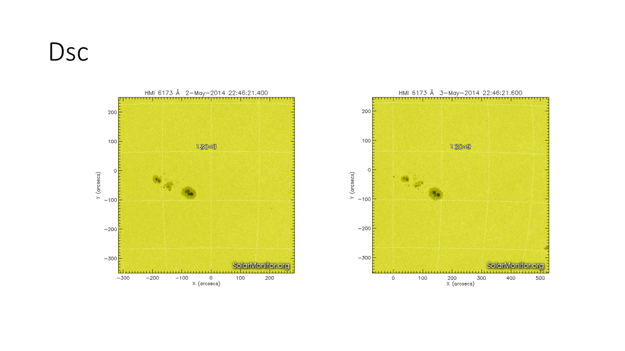
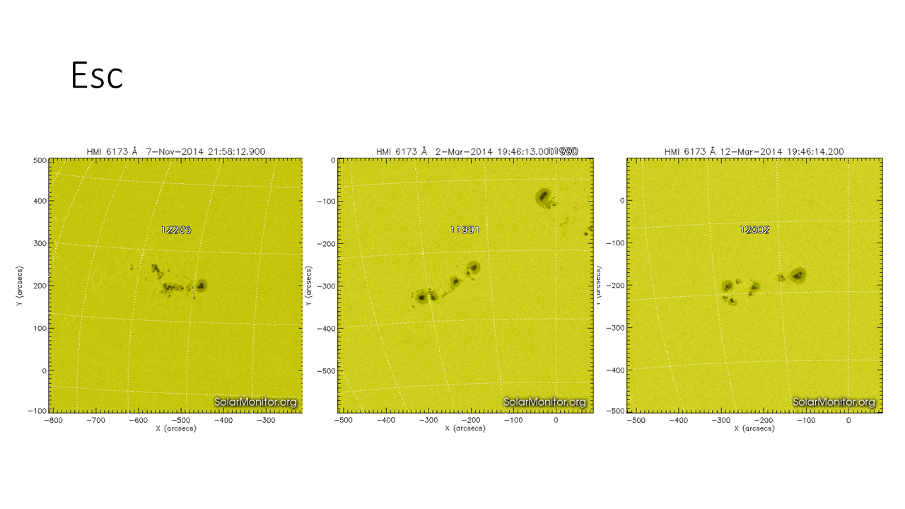
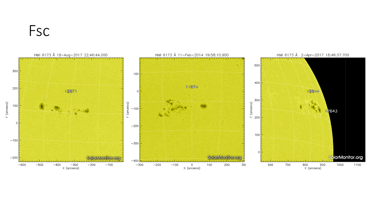
| Dsc | Esc | Fsc | |||
| Dac | Eac | Fac | |||
| Hhx | Cho | Dho | Eho | Fho | |
| Chi | Dhi | Ehi | Fhi | ||
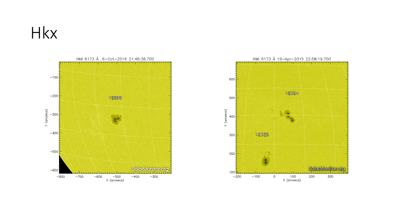
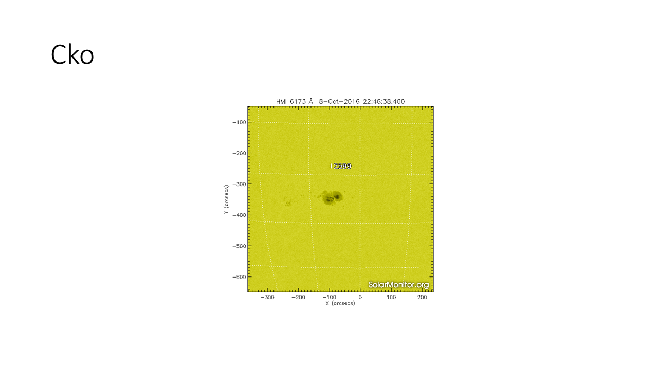
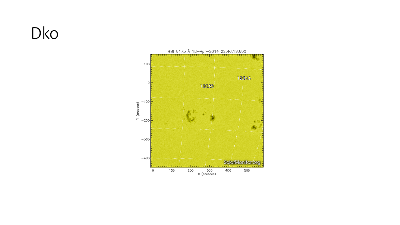
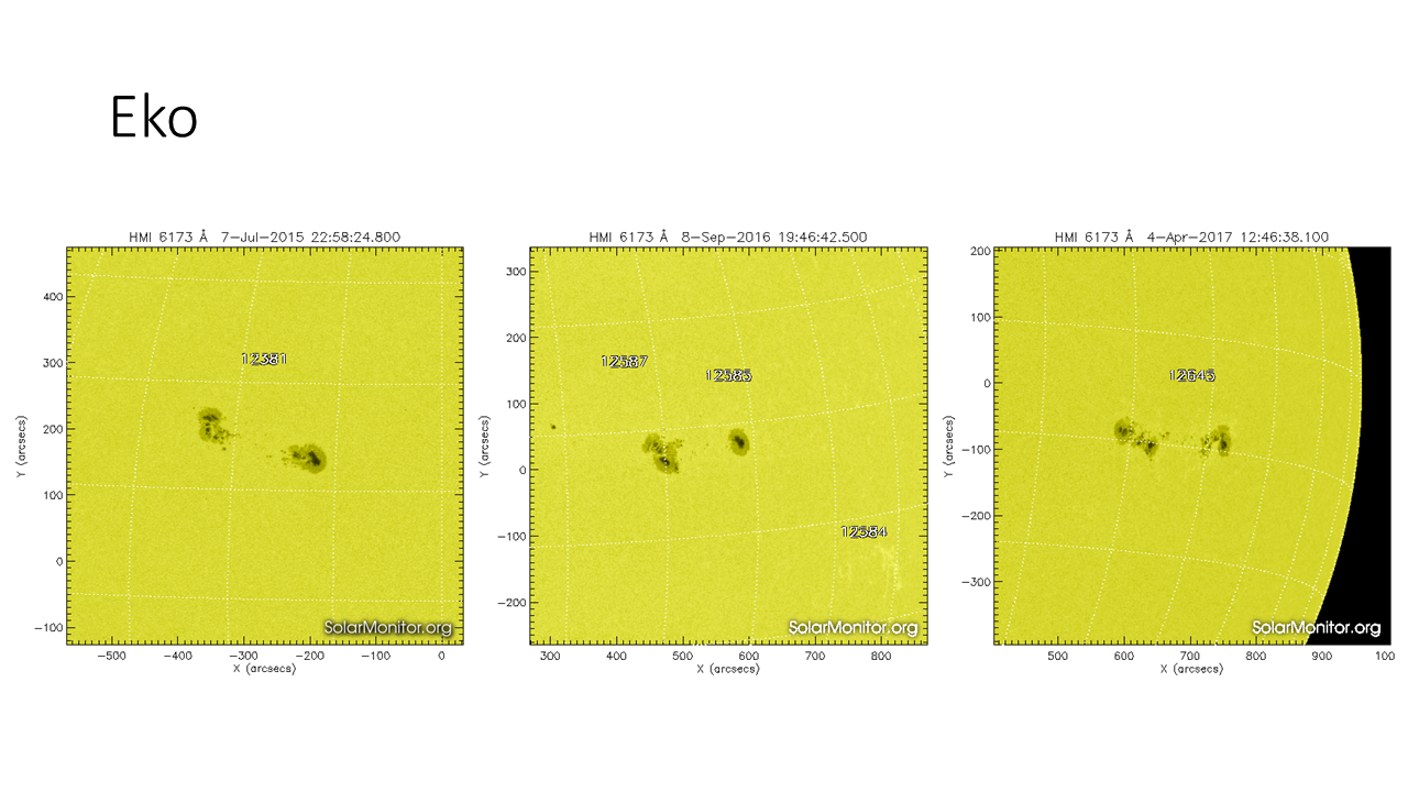
| Hkx | Cko | Dko | Eko | Fko | |
| Cki | Dki | Eki | Fki | ||
| Dhc | Ehc | Fhc | |||
| Dkc | Ekc | Fkc |
Mount Wilson Magnetic Classification
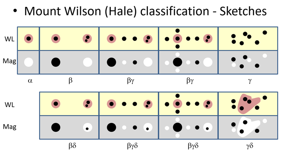
Sunspot regions can also be classified according to the magnetic polarities of their sunspots. A classification scheme was first developed by Hale et al. (1919) and later expanded by Künzel (1965). The classification that is currently in use contains the 4 basic magnetic types as introduced by Hale, with the 3 more complex classes having the possibility to be appended by the suffix "delta" as devised by Künzel. "Delta spots" are notorious for producing significantly more and stronger flares than the other groups. When classifying sunspot groups according to the Mount Wilson scheme, one should be aware of any line-of-sight effects if the region is located close to the solar limb.
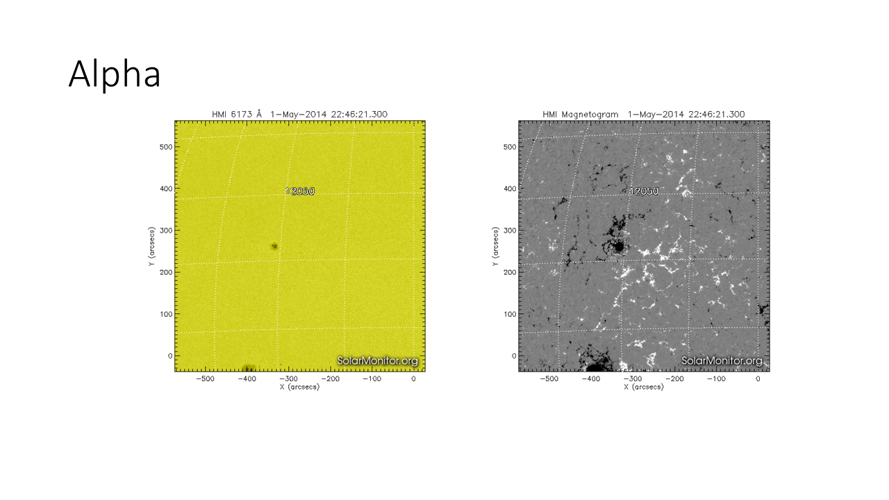
Alpha - Denotes a unipolar sunspot group, i.e. single spots, or groups of small spots, having the same magnetic polarity. It should be noted, however, that unipolar spots, and the chief components of bipolar groups, may occasionally have small companions of opposite polarity, which play such a minor and sporadic part in the group that they are disregarded in the classification. EXAMPLES
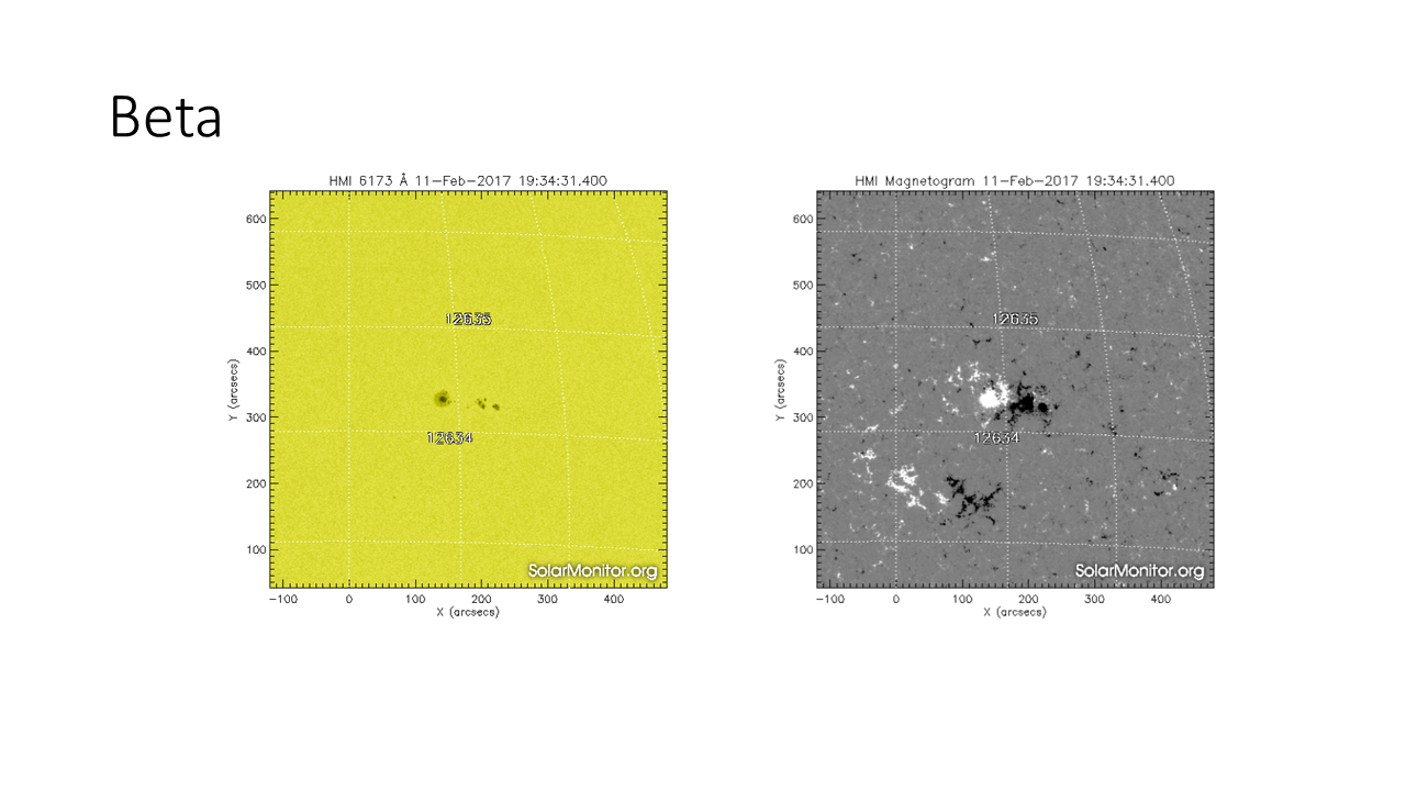
Beta - The simplest and most characteristic bipolar sunspot group consists of two spots of opposite magnetic polarity. The line joining the two spots generally makes only a small angle with the solar equator. Each member of the group may be accompanied or replaced by many small spots, but the great majority of the spots constituting the preceding and following members of the group are of opposite magnetic polarity. One or more companion spots, of polarity opposite to that which characterizes the corresponding region of the group, sometimes occur in association with either the preceding or following member. The positive-negative polarity inversion line is clear and simple. EXAMPLES
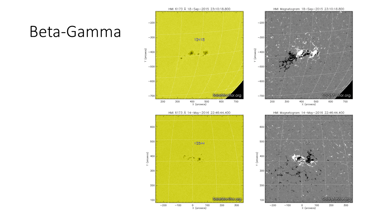
Beta-Gamma - Bipolar sunspot groups in which the preceding or following members are accompanied by minor spots of opposite magnetic polarity. The positive-negative polarity inversion line is complex (e.g. "wavy") or the sunspot region may contain more than 1 clear inversion line. EXAMPLES
Gamma - This concerns multipolar sunspot groups, i.e. groups containing spots of both polarities so irregularly distributed as to prevent classification as bipolar groups.
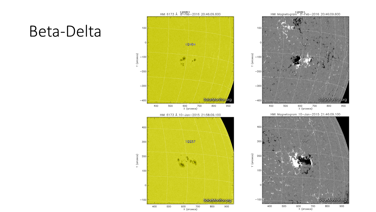
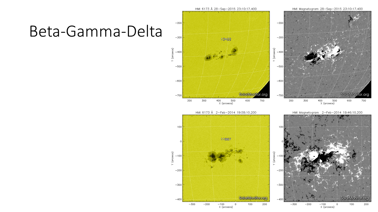
Delta - A suffix that can be appended to the beta, beta-gamma, and gamma classes if the sunspot group contains at least one mature spot in which umbrae of opposite polarities are separated by less than 2° and situated within the common penumbra. Delta regions have a much higher flaring probability than the other regions. EXAMPLES: Beta-Delta , Beta-Gamma-Delta
Thus, the Mount Wilson classification contains 7 possible classes (the links above provide some examples): A, B, BG, G, BD, BGD and GD. A sketch depicting the different classes can be found underneath. For the period 1992-2015, the beta groups are the most numerous (64%) followed by the alpha regions (20%), beta-gamma (11%), beta-gamma-delta (4%), and beta-delta (1%) (Jaeggli and Norton 2016). The gamma and gamma-delta classes are extremely rare (less than 0,05%). Sunspot regions containing a delta spot are about 3 times more flare-prone than the G and BG groups, and about 10 times more than the A and B groups (Shin et al. 2016).
X-ray flare classification
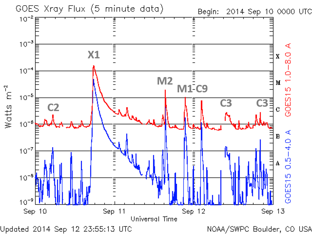
Solar flares can be ranked according to the peak energy output in x-ray. These measurements have been systematically carried out since 1976 by the GOES satellites. The scheme was developed by Don Baker for NOAA during the mid-1960s (Poppe and Jordan, 2006). He used the wavelength band from 1 to 8 Angstrom (0.1-0.8 nm), as these wavelengths seemed to best characterize a flare's intensity. The scheme was labeled "CMX": C, M, and X stand for small (or "Common"), Medium, and large (or "eXtreme") flares. The range was logarithmic, each class being 10 times stronger than the previous one, and within each category ranging from 1 to 9 (e.g. a C9 flare, an M3 flare,...). As the instruments over the subsequent years became more sensitive, smaller flares could be observed which were then labeled A and B. Similarly, Y and Z could follow X if X10 or stronger flares were detected, but these have never been used. Instead, scientists continued the X-class for labeling very large flares, and so the strongest flare so far observed by the GOES satellites is an X28 (and not an Y2.8). Note the peak intensity of a flare is based on the 1-minute averages by GOES, not on the 5-minute averages which are often used for the graphs. Also, the peak intensity may not be rounded up, as the true flux never reached that level (e.g. a C5.8 is a C5 flare, not a C6 event).
The annotated scheme underneath shows the GOES x-ray flux as available on the dedicated NOAA/SWPC website, with the intensities of some flares indicated. Thus, a C3 event for example, indicates an x-ray burst with 3x10⁻⁶ W/m2 peak flux. The subsequent table links the classes to the corresponding x-ray flux intensity I (0.1 - 0.8 nm, and expressed in Watt per square meter, W/m2).
| Class | Peak (W/m2) |
| A | I < 10-7 |
| B | 10-7 ≤ I <10-6 |
| C | 10-6 ≤ I <10-5 |
| M | 10-5 ≤ I <10-4 |
| X | 10-4 ≤ I |
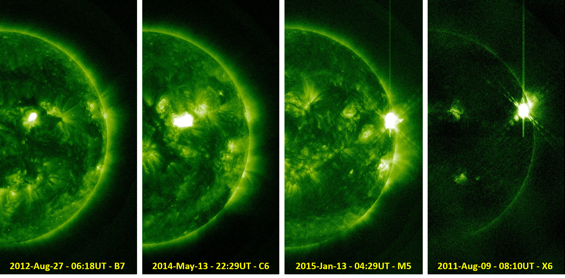
The composition underneath gives an idea for each class how a flare looks like in extreme ultraviolet. The images were taken by the Solar Dynamics Observatory (SDO) near the time of the maximum x-ray intensity. The X-class flare was so bright that it triggered the ‘active exposure control’ algorithm to compensate for the extra light coming in from a flare. This algorithm creates a shorter exposure time, and thus a dimmer, but still scientifically useful view of the Sun (Chamberlin et al., 2012).
Levels of solar activity
The levels of solar activity are based on the number and strength of flares observed by the GOES satellite in the 0.1-0.8 nm band over 24 hours (usually the previous day). Devised by NOAA/SWPC and in use by most SWx centres, the terminology is as shown in the table underneath.
| Terminology | Description |
| Very low | No flares, or flaring events of A- or B-class x-ray level only |
| Low | C-class x-ray events |
| Moderate | Isolated (one to four) M-class x-ray events |
| High | Several (5 or more) M-class x-ray events, or isolated (one to four) M5 or greater x-ray events |
| Very high | Several (5 or more) M5 or greater x-ray events |
In the annotated x-ray graph underneath, solar activity on 10, 11 and 12 September 2014 was respectively high (1 flare greater than M5), moderate (two low-level M-class flares), and low (only C-class flares).
Optical flare classification
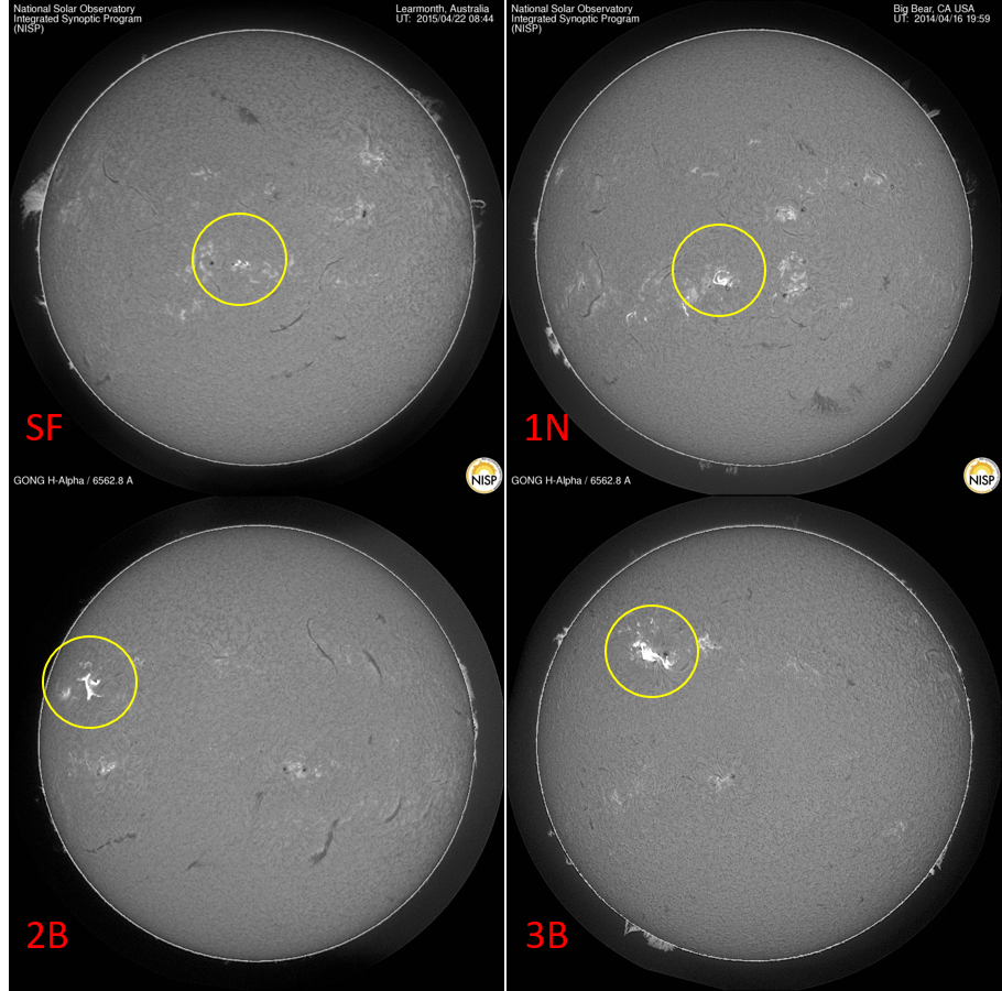
Flares can also be classified according to their size and brightness in H-alpha, a line at 656.28 nm in the red part of the solar spectrum. This optical system was approved by Commission 10 of the IAU and came in effect on 1 January 1966. It consists of a dual code: the importance of the flare which is based on the flare area, and the brightness of the flare.
The importance of the flare is its area determined at the maximum brightness of the flare (not its maximum size) and is expressed in heliocentric square degrees. The area needs to be corrected for line-of-sight effects (projection), but height effects make the areas of flares located more than 65 degrees from the central meridian quite inaccurate (e.g. Falciani et al. 1967). As outlined in the table underneath, 5 importance classes can be assigned pending the obtained area: S (for "subflare"), 1, 2, 3 and 4.
|
Area (square degrees) |
Area (10-6 solar disk*) |
Importance class |
Typical corresponding soft x-ray class |
| < 2.0 | < 200 | S | C2 |
| 2.1 - 5.1 | 200 - 500 | 1 | M3 |
| 5.2 - 12.4 | 500 - 1200 | 2 | X1 |
| 12.5 - 24.7 | 1200 - 2400 | 3 | X5 |
| > 24.7 | > 2400 | 4 | X9 |
* : millionths of the total area of the solar disk. If one wants to express the area in millionths of a solar hemisphere (MH), the values have to be halved, thus ranging from < 100 MH (S) to > 1200 MH (4). See respectively Zirin (1988) and AFWAMAN 15-1 (2013).
The brightness of a solar flare can be determined in two ways, as described in the manuals of the Air Force Weather Agency (AFWAMAN 15-1 (2013), Wittman (2012), Giersch (2016) and on the website from the Australian space weather service (SWS).
When photometry is available (either photographic or digital), the so-called automatic mode, a flare may be classified into one of three categories: F (faint), N (normal) or B (brilliant), according to the peak brightness of any area which exceeds 10 millionths hemispheric area, as specified in the table below. Note that the background chromospheric intensity should be measured in the same general area of the flare to compensate for limb darkening effects. So, if a flaring region reaches a brightness of 1.6 times (160%) the surrounding quiet sun background brightness, then it is considered a faint (F) flare. If the flaring region reaches a brightness between 260% and 360% the background brightness, it is catalogued as a flare of normal intensity (N). Finally, in order to be considered a "brilliant" flare (B), the flaring region should reach an intensity of 360% the background brightness and its are should cover at least 10 millionths of the solar hemisphere.
If photometry is not available, a semi-automatic procedure can be applied in which the H-alpha filter can be tuned off-band (i.e. away from its centre line at 656.28 nm). In such a case, the total bandwidth of the most brilliant parts of the flare may be used as a surrogate to try and estimate the brightness category. Thus, in order to classify a flare as faint (F), it should be distinctly visible as an enhanced area over a line width of 0.08 nm or greater, but less than 0.12 nm. This bandwidth may be asymmetrically displaced around the H-alpha line centre (eg, from +0.02 to -0.06 nm). If the flare is visible over a bandwidth more than 0.12 nm but less than 0.2 nm, its intensity is classified as "normal" (N). Finally, if the flare is visible over a band of 0.2 nm or more, its intensity is catalogued as "brilliant" (B). In this semi-automatic mode, the 10 MH requirement is waived for N and B thresholds and the off-band measurement is sufficient.
| Brightness class | Automatic (% of Background) | Semi-automatic (total bandwidth) |
| F (faint) | 160% < brightness < 260% | 0.08nm < bandwidth < 0.12 nm |
| N (normal) | 260% < brightness < 360% | 0.12nm < bandwidth < 0.2 nm |
| B (Brilliant) | brightness > 360% | bandwidth > 0.2 nm |
The optical classification of a flare is then obtained by combining its importance (5 classes) with its brightness (3 classes), thus allowing for 15 possibilities ranging from SF (most numerous) to 4B (extremely rare). Annotated examples of flares classified as SF, 1N, 2B and 3B can be found underneath (images from NSO/GONG). It's followed by an example of a 4B flare can be found here (from Ambastha 2007). It concerns the X17 flare from 28 October 2003 as observed by the H-alpha instruments from the Udaipur Solar Observatory.
Radio emission storms
The Sun also emits in the radio domain, with frequencies ranging from THz to kHz. Ground-based radio observations are limited by the ionospheric critical frequency (foF2 , also known as cut-off frequency) to 10-20 MHz, and therefore satellite measurements such as from STEREO-A/WAVES are required to observe the solar radio emissions below these frequencies. Using a spectrograph, a dynamic spectrum can be created showing the evolution of the emission of the whole Sun in the frequency-time plane. Underneath is such a diagram, with time in minutes on the horizontal axis, and the frequency on the vertical axis (logarithmic). In the sketch underneath, the vertical axis shows decreasing frequencies in the upward direction, corresponding to increasing distances from the solar surface. The sketch depicts 5 typical disturbances observed in a radio spectrogram, labelled Type I to Type V (Wild 1963). For SWx purposes, only Type II, III and IV bursts are of importance The descriptions below were taken from various sources: White (2007) ; Gopalswamy (2011) ; Karlicky (2017). The examples were selected from the Humain Radioastronomy Station at and from the e-CALLISTO / Trieste network. Please mind the scaling of the axes.
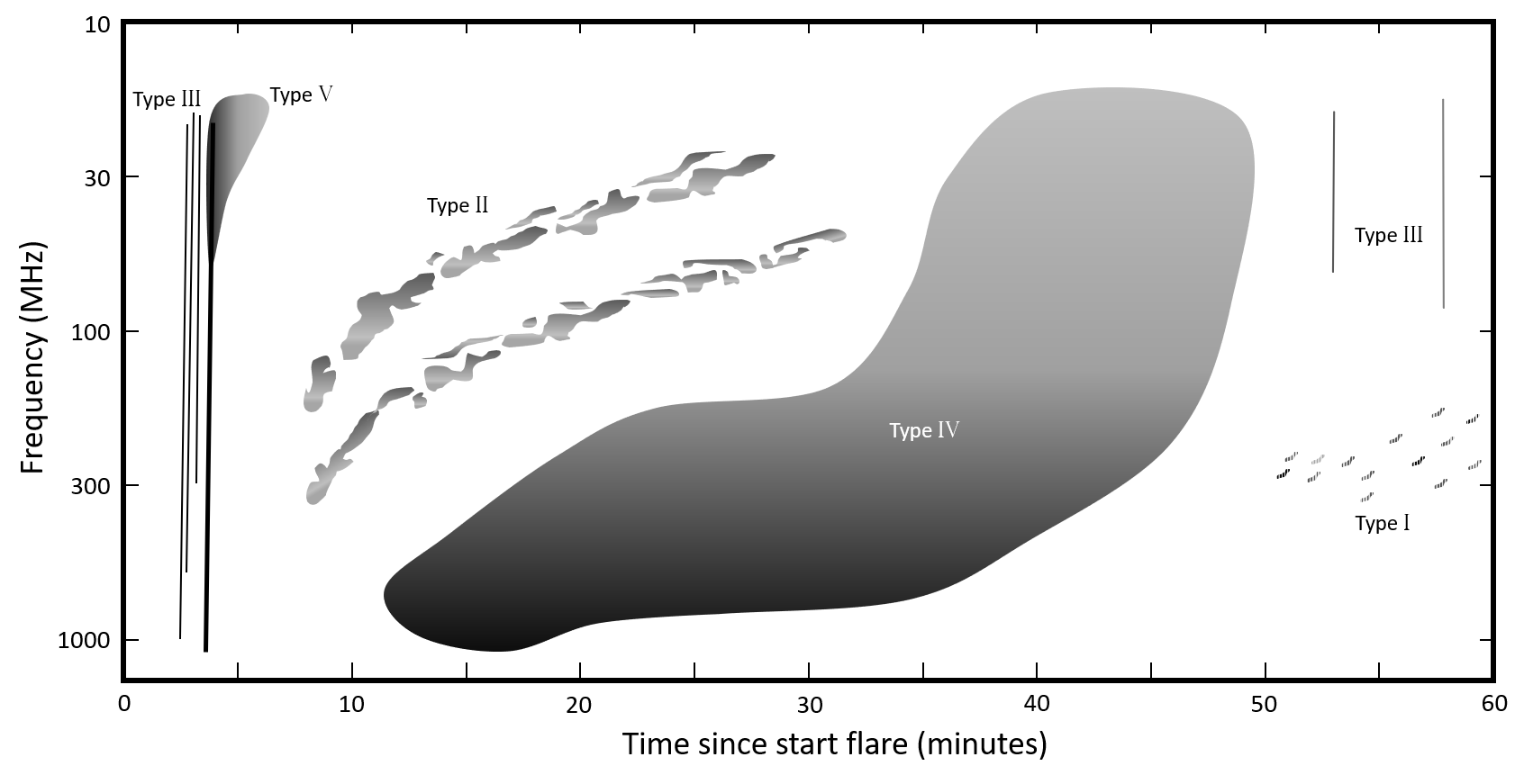
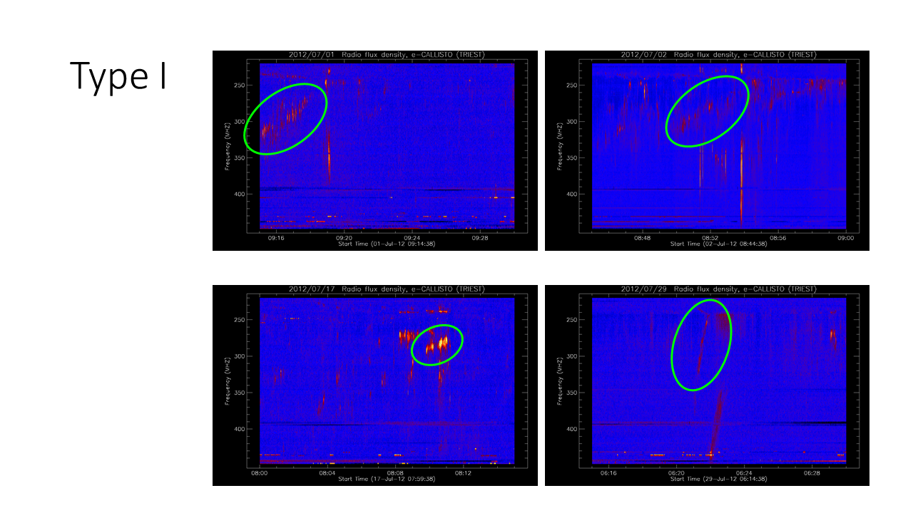
Type I - Type I radio bursts are quite common and non–flare–related phenomena observed in the frequency range 100–400 MHz, consisting of a continuum component and a burst component. They last from a few hours to several days and are associated with the active region passage over the solar disc. The long duration of the continuum emission ("noise storm") suggests that it is due to energetic electrons trapped on closed coronal magnetic field lines. The associated Type I bursts are brief (order of seconds) and very narrow band (several MHz), appearing in drifting chains ("clouds") of short duration (minutes) and narrow bandwidth bursts (10-20 MHz), superimposed on a broadband continuum. These chains preferentially drift towards lower frequencies and their drift is used for estimations of the magnetic field in their sources (active regions, prominences). EXAMPLES
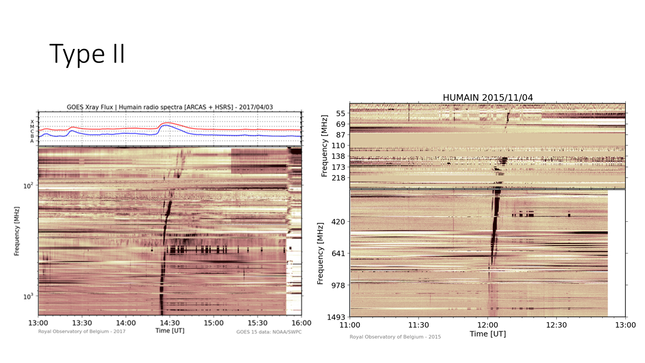
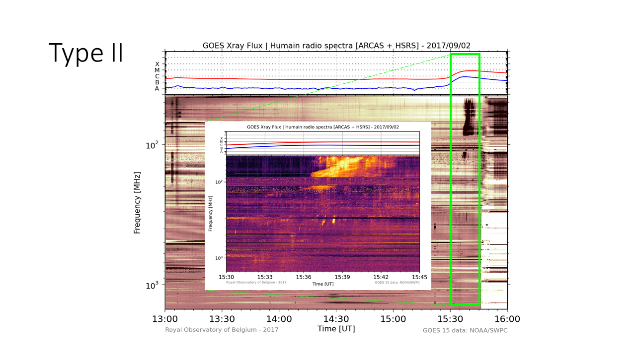
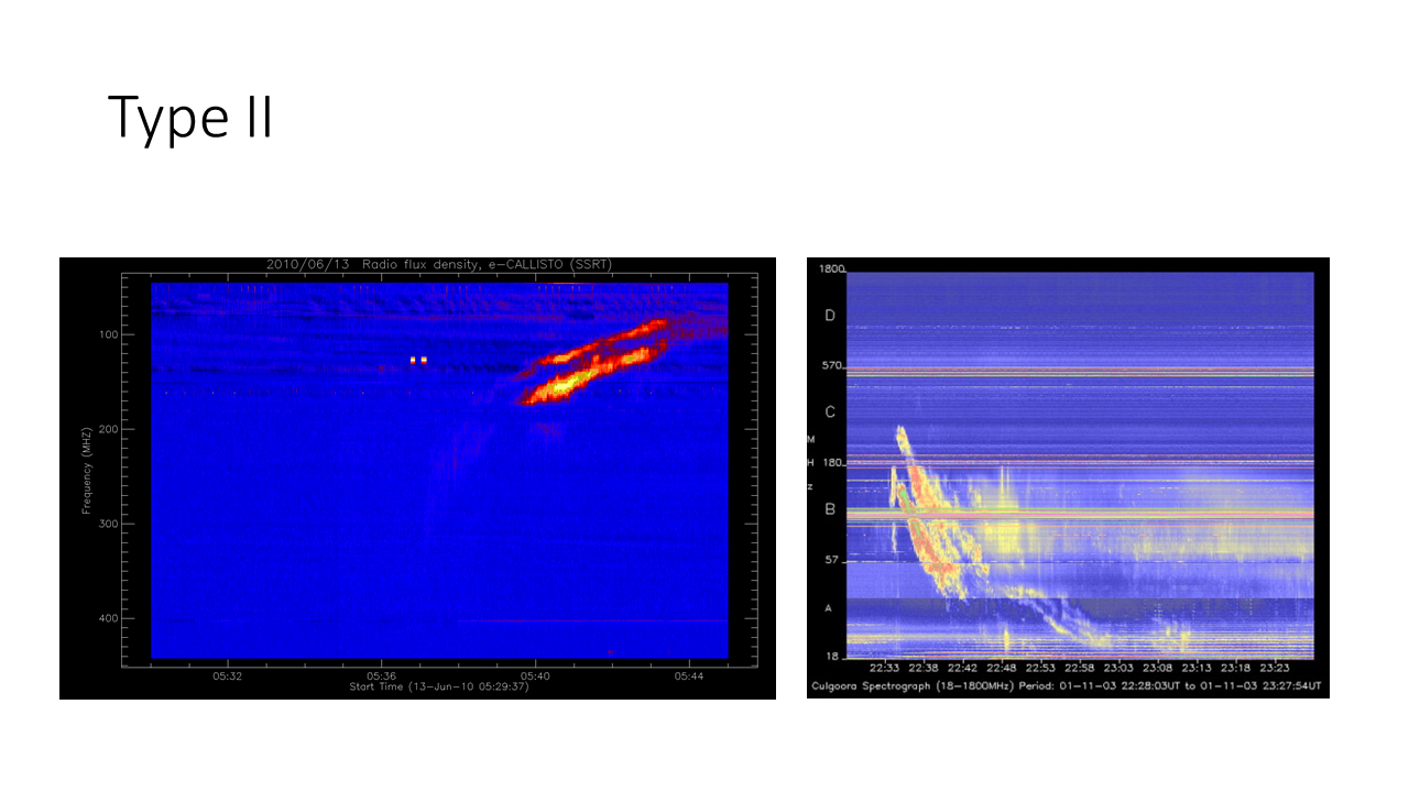
Type II - Type II bursts typically start around the time of the soft X–ray peak in a solar flare and are identified in dynamic spectra by a slow drift of narrow-band emission to lower frequencies with time (from about 300 MHz to about 20 MHz). There's also a frequent presence of both fundamental and second–harmonic bands (with a frequency ratio of 2), and often a splitting of each of these bands into two traces. The frequency drift rate is typically two orders of magnitude slower than that of the (“fast–drift”) Type III bursts, so the two burst types are readily distinguished. Type II bursts are produced by electrons accelerated by CME-driven shocks in the corona. Even X-class flares are not associated with type II bursts if they lack CMEs. The shock speed of the CME is calculated from the fundamental band (the one with the lowest frequencies). EXAMPLES 1 - 2 - 3
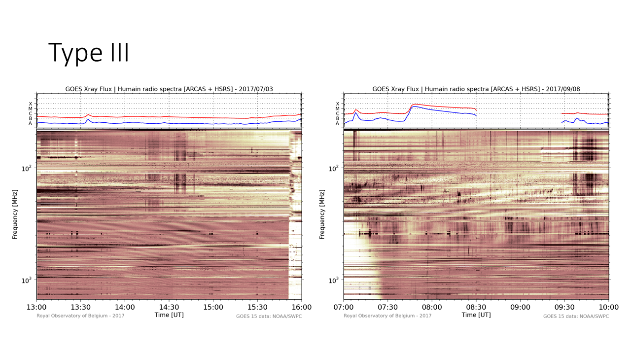
Type III - Type III bursts are brief radio bursts in the 1GHz-10kHz range that drift very rapidly in frequency versus time. For example, it can drift from 50 to 20 MHz in about 3 seconds, or 10 MHz/s. Type III bursts are thought to be produced by electron beams propagating along open magnetic field lines via the plasma emission mechanism. There are three low-frequency variants of type III bursts that originate in the interplanetary medium: (i) isolated type III bursts from flares and small-scale energy releases, (ii) complex type III bursts during CMEs, and (iii) type III storms. In addition to isolated or groups of bursts, Type IIIs are commonly seen in the impulsive phase of solar flares, and the connection they imply between the acceleration region in solar flares and open field lines that reach the solar wind makes them important for understanding field line connectivity in flares and the access of flare–accelerated particles to the Earth. EXAMPLES
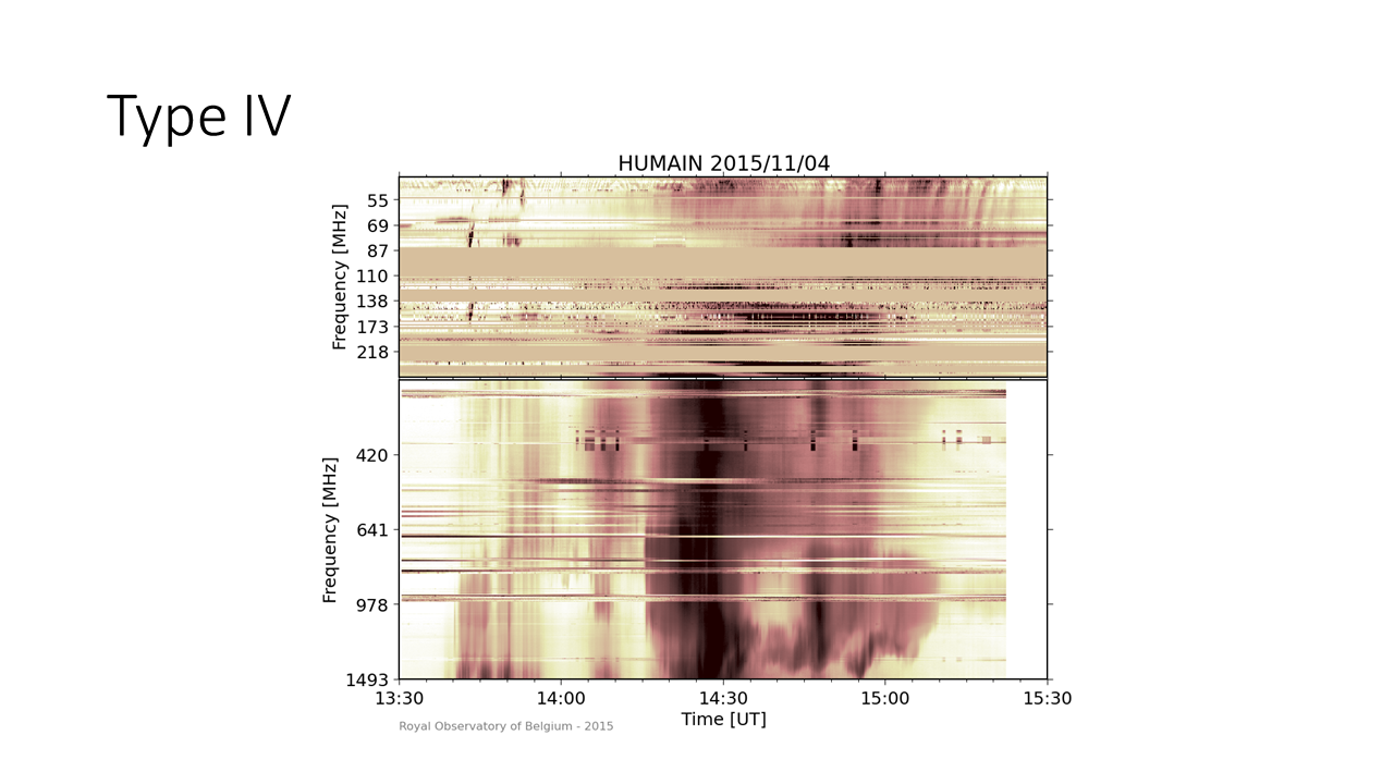
Type IV - Type IV bursts are broadband (2GHz - 20 MHZ) quasi–continuum features associated with the decay phase of solar flares, and can last for several hours. They are attributed to electrons trapped in closed field lines in the post–flare arcades produced by flares; their presence implies ongoing acceleration somewhere in these arcades, possibly at the tops of the loops in a "helmet–streamer" configuration. Although they are not as common as Type II and III bursts, Type IV bursts are of interest in SWx studies because they are strongly associated with solar energetic particle events. EXAMPLES
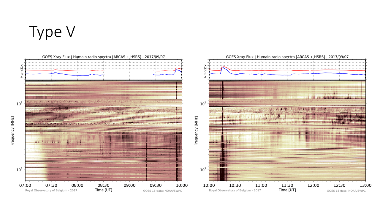
Type V - Associated with Type III bursts are the last of the original classes of radio bursts, Type V. The Type V emission is a longer–duration (1-3 minutes) low–frequency (10-200 MHz) component that looks to be "attached" to (and possibly emerging from) the decay phase of the Type III burst ahead of it. Type V bursts are often difficult to identify, particularly if there are other bursts present at the same time. They are relatively rare and have no known SWx implications. EXAMPLES
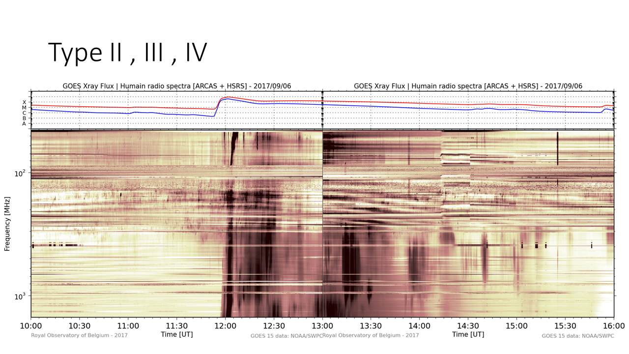
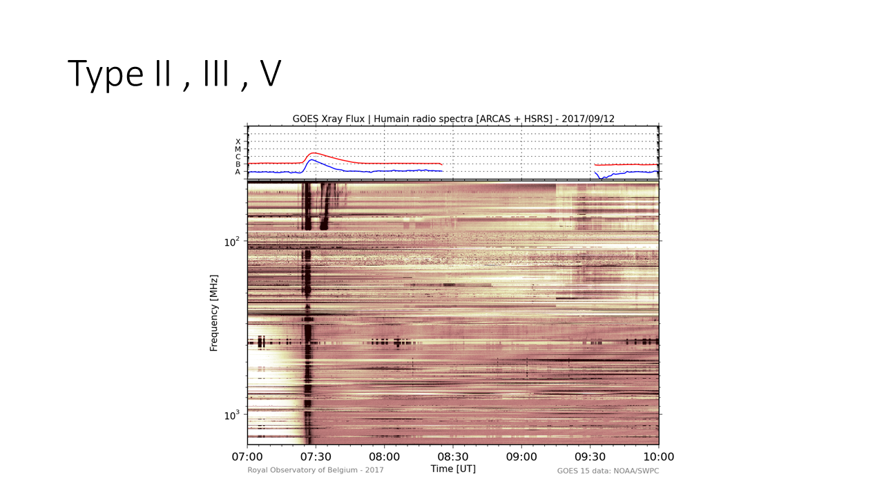
Underneath two radio spectra that combine a number of radio types: Types II, III, and IV on 6 September 2017, and Types II, III and V on 12 September 2017.
NOAA/SWPC also uses three other types of bursts in their event reports:
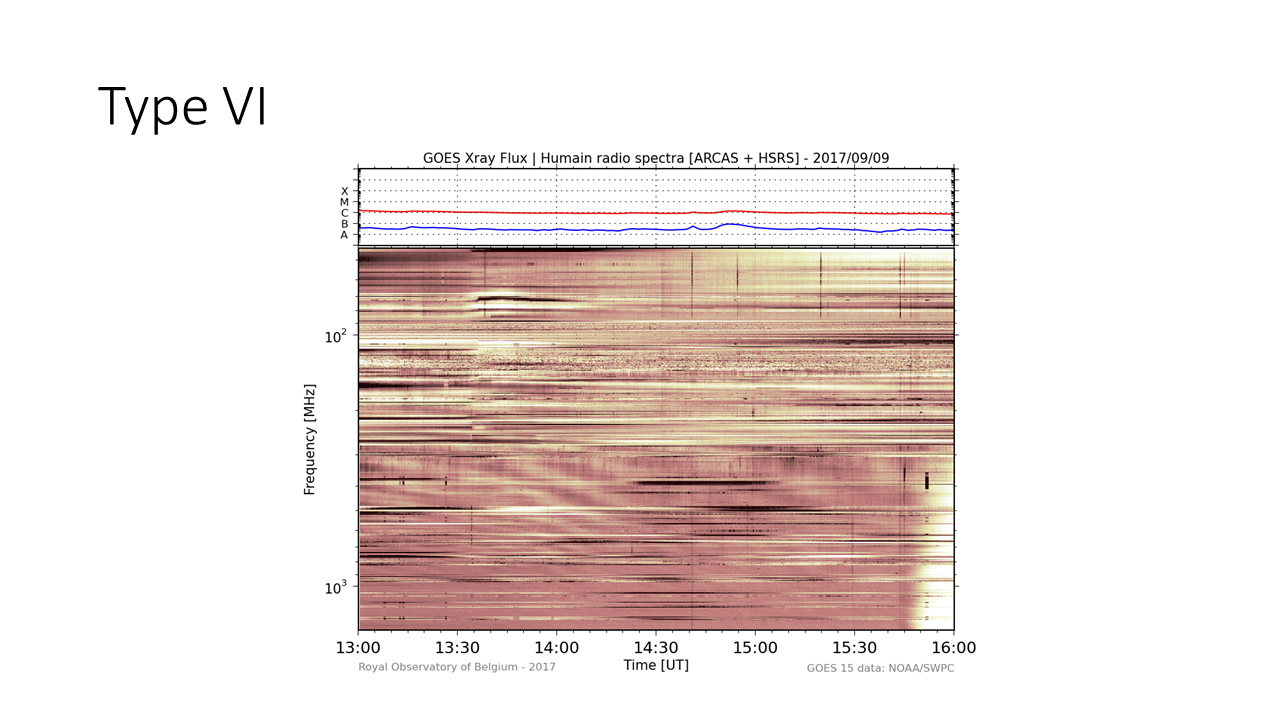
- Type VI: series of Type III bursts over a period of 10 minutes or more, with no period longer than 30 minutes without activity. EXAMPLE
- Type VII: series of Type III and Type V bursts over a period of 10 minutes or more, with no period longer than 30 minutes without activity.
- Type CTM: A broad-band decametric continuum emission. The tag CTM is an abbreviation for continuum storm used in GOES reports. It indicates solar radio noise which can last from hours to days.
The type of the observed radio burst is often supplemented by a qualifier 1, 2 or 3, such as III/1 or II/3. This suffix relates to the intensity of the burst in a relative scale: 1=Minor ; 2=Significant ; 3=Major.
Geomagnetic Indices
The main purpose of geomagnetic indices is to objectively quantify the level of perturbations of the earth's magnetosphere. They are simple measures of magnetic activity that occurs, typically, over periods of time of less than a few hours and which is recorded by magnetometers at ground-based observatories. Various indices have been developed, and this section is limited to those indices most often used in the SIDC SWx bulletins and URSIgrams. The description of the indices is in large part based on Perrone and De Franceschi (1998) ; Love and Remick (2007) ; Matzka et al. (2021), and from the ISGI website.
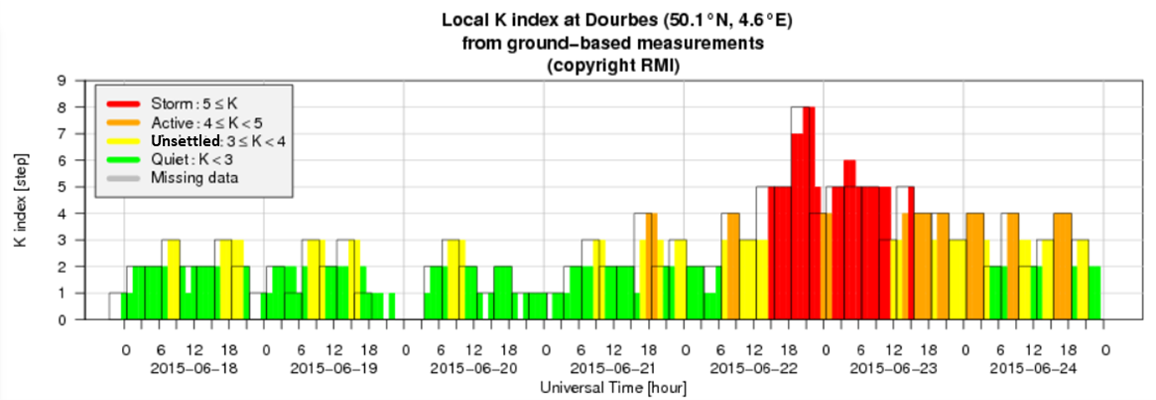
K index - The K index (K stands for "Kennziffer") is a 3-hourly quasi-logarithmic local index of geomagnetic activity relative to an assumed quiet-day curve for the recording site. The observations measure the deviation (minimum-to-maximum amplitude) of the most disturbed horizontal component, and are corrected for diurnal and seasonal changes. A scaling is done such that the historical number of disturbances at a certain K-level are about the same at all stations, thereby also removing the latitudinal effect. The K index ranges from 0 to 9 (dimensionless integer). It was introduced by Bartels in 1938 and Bartels et al. in 1939. Note the K index is a local index, and as such often the subscript "k" is used to indicate the individual station, e.g. pending the context, KD, KDO, KDOUR, ... may all refer to the Dourbes K index. Underneath a graph showing the evolution of the K index at Dourbes during one of the strongest geomagnetic storms of solar cycle 24, on 22-23 June 2015. The colored bars in the K_BEL and K Dourbes indices are hourly updated K values, calculated from data over the previous 3 hours, e.g. The value declared at 10:00UT is based on data over the timerange 7:00-10:00UT. The transparent bars are the 3-hourly values at the typical intervals, i.e. at 03:00UT for the interval 00:00-03:00UT, at 06:00UT for the interval 03:00-06:00UT, and so on.
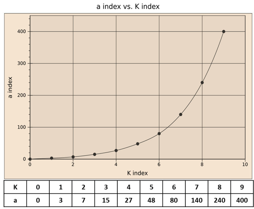
ak index - The local K index is a quasi-logarithmic index, and as such averages cannot be taken. This poses a problem when one wants to express geomagnetic activity over e.g. a day or a month. To this aim, a 3-hourly "equivalent amplitude" index of local geomagnetic activity was established, with "ak" related to the 3-hourly K index according to the scale underneath. Also here, the subscript "k" used in ak refers to the individual station "k".
Ak index - The Ak index for a station "k" is simply the average of the eight ak indices for that station for the UT day. The subscript "k" used on the Ak refers to the individual station, e.g. pending the context, AD, ADO, ADOUR, ... may all refer to the Dourbes A-index.
Kp index - So far, we have only been discussing the local geomagnetic indices. The Kp index ("planetarische Kennziffer") is a 3-hourly geomagnetic range index averaged from the *standardized* local K indices of 13 contributing subauroral geomagnetic observatories worldwide (list at ISGI). To distinguish the 3-hourly from the daily values, it is common practice to use resp. kp and Kp. Note that because of the historical context at the time of its creation, the Kp network is heavily weighted towards Europe and Northern America). Building on earlier work in the late 1930s and early 1940s, it was introduced by Bartels in 1949 (The standardized index Ks and the planetary index Kp, IATME Bulletin 12b, 97), and extended further back in time to 1932. The scale is open-ended, i.e. no matter how large the geomagnetic variation is, Kp will never exceed 9 (9o). The well-known charts published on the NOAA/SWPC website concern the Estimated Kp, i.e. a preliminary Kp based on only 8 geomagnetic stations and expressed in thirds of an integer from 0 to 9. The final 3-hourly and daily Kp indices are compiled by GFZ Potsdam and also expressed in thirds, from 0o, 0+, 1-, ... to 9-, 9o. The final Kp values are archived at the World Data Center for Geomagnetism at Kyoto (WDC Kyoto). The Kp index is also used by NOAA as the base physical parameter for their G-scale (NOAA/SWPC scales), describing common SWx effects from geomagnetic storms and associated with Kp levels of 5 or higher (Poppe (2000).
ap index - To solve the averaging issue with the Kp indices, The 3-hourly ap (equivalent range) index is derived from the Kp index in accordance with the table underneath. The "p" refers to "planetarische", to clearly distinguish the planetary character of the ap index as compared to the local ak index.
| Kp | 0o | 0+ | 1- | 1o | 1+ | 2- | 2o | 2+ | 3- | 3o | 3+ | 4- | 4o | 4+ |
| ap | 0 | 2 | 3 | 4 | 5 | 6 | 7 | 9 | 12 | 15 | 18 | 22 | 27 | 32 |
| Kp | 5- | 5o | 5+ | 6- | 6o | 6+ | 7- | 7o | 7+ | 8- | 8o | 8+ | 9- | 9o |
| ap | 39 | 48 | 56 | 67 | 80 | 94 | 111 | 132 | 154 | 179 | 207 | 236 | 300 | 400 |
Ap index - The Ap index is simply the average of the eight ap indices for the UT day. The "p" refers to "planetarische", to clearly distinguish the planetary character of the Ap index from the local Ak index.
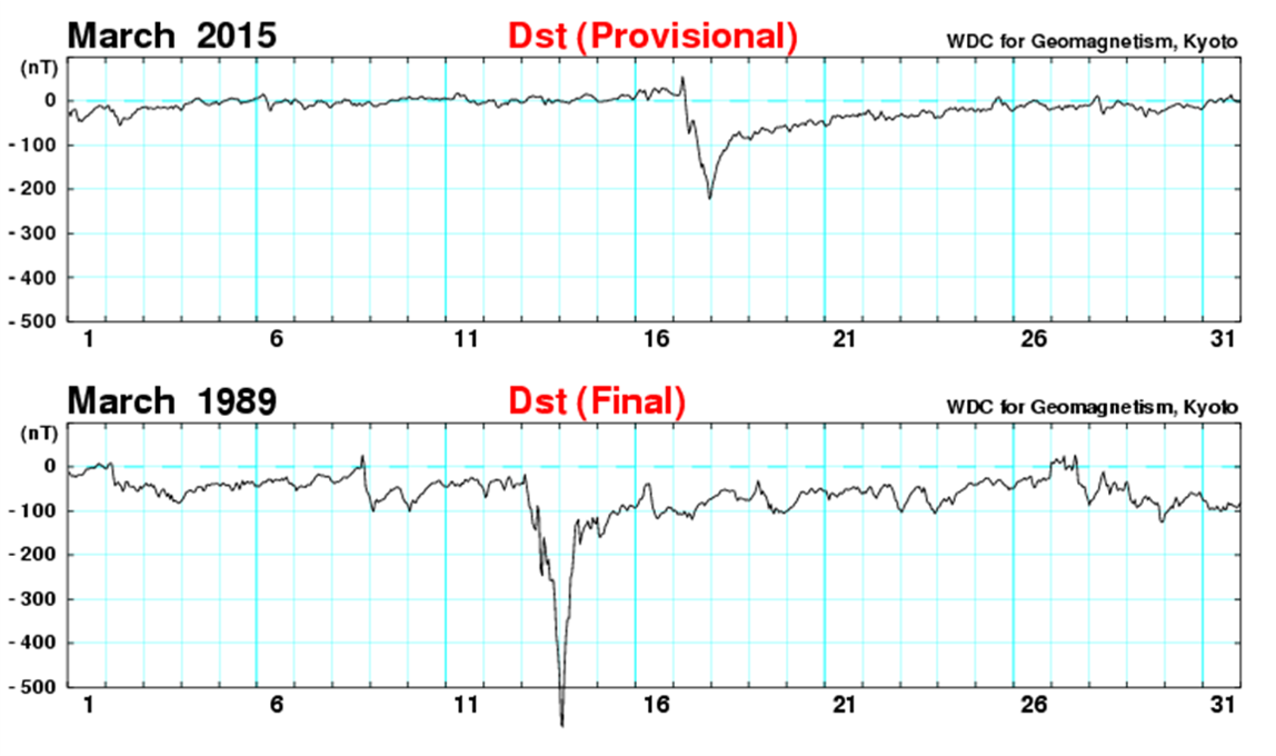
Dst index - The Disturbance storm-time index Dst (Sugiura, 1964) is designed to measure the magnetic signature of magnetospheric currents, in particular -but not restricted to- the ring current. Dst is computed using 1-hour values of the horizontal H-component by four low latitude observatories (list at ISGI) sufficiently distant from the auroral and equatorial electrojets to inhibit noise from these two sources. The values are expressed in nT and mostly negative in case of a strong geomagnetic disturbance, as the enhanced ring current tends to counteract (weaken) the earth's magnetic field. The Dst index is derived and maintained by the World Data Center for Geomagnetism at Kyoto, Japan (WDC Kyoto). Underneath two examples showing the evolution of the Dst following a strong disturbance: The St-Patrick's day storm, which was the strongest geomagnetic storm of solar cycle 24, and the famous geomagnetic storm from 13-14 March 1989 which resulted in the Québec power grid failure.
Levels of geomagnetic activity
The following terminology is based on the Ap and Kp indices and used to describe global geomagnetic activity. As such , they can also be applied to other geomagnetic indices described in the previous paragraph such as ap and kp, and in extenso also to ak, Ak, k, and K. The terminology is being used by a large number of SWx centers, including the SIDC, K_BEL, and K Dourbes. It also conforms to the NOAA/SWPC G-scale.Local magnetometer stations or dashboards from the various SWx institutes may use (slightly) different terms. Best and safest practice is to check the numbers!
| Terminology | Ap range | Kp range | K |
| Quiet | 0 < Ap < 10 | 0o < Kp < 2+ | 0, 1, 2 |
| Unsettled | 10 < Ap < 20 | 3- < Kp < 3+ | 3 |
| Active | 20 < Ap < 35 | 4- < Kp < 4+ | 4 |
| Minor storm | 35 < Ap < 60 | 5- < Kp < 5+ | 5 |
| Moderate storm | 60 < Ap < 100 | 6- < Kp < 6+ | 6 |
| Strong / Major storm* | 100 < Ap < 160 | 7- < Kp < 7+ | 7 |
| Severe storm | 160 < Ap < 310 | 8- < Kp < 9- | 8 |
| Extreme storm | 310 < Ap < 400 | Kp = 9o | 9 |
* : SIDC and K_BEL / K Dourbes use the term "Major storm", whereas "Strong storm" is used in e.g. the NOAA G-scale.
Of note is that ISES, the overarching International Space Environment Service, uses a coarser terminology in its encoded messages. ISES is a collaborative network of space weather service-providing organizations around the globe, currently including 20 Regional Warning Centers such as e.g. SWPC and the SIDC at the Royal Observatory of Belgium, who conform to this code in their coded bulletins. The table underneath summarizes the terminology used.
| ISES code | ISES | SIDC | A range | K index |
| 0 | Quiet | 0 < A < 20 | K < 4 | |
| 1 | Active | 20 < A < 30 | K = 4 | |
| 2 | Minor storm | 30 < A < 50 | K = 5 | |
| 3 | Moderate storm | 50 < A < 100 | K = 6 | |
| 4 | Severe storm | Major storm | 100 < A | K > 7 |
Geomagnetic conditions can also be described based on the Dst index. Please remember that a more negative Dst index means a stronger geomagnetic disturbance. Two main schemes are in place: One described by Gonzales et al. (1994) and Echer et al. (2013), the other by Loewe et al. (1997) and Borovsky et al. (2017). They are similar in terminology and levels, and differ mostly in view of the statistics and purpose of the research. In the examples given in the preceding paragraph, the 17 March 2015 storm and the 13-14 March 1989 storm can be labeled respectively as an intense storm and an extreme storm according to the Gonzales et al. scheme.
| Gonzales et al. (1994) and Echer et al. (2013) | Loewe et al. (1997) and Borovsky et al. (2017) | ||
| Terminology | Dst range (nT) | Terminology | Dst range (nT) |
| Quiet | Dst > -30 | Quiet | Dst > -30 |
| Weak storm | -50 < Dst < -30 | Weak storm | -50 < Dst < -30 |
| Moderate storm | -100 < Dst < -50 | Moderate storm | -100 < Dst < -50 |
| Intense storm | -250 < Dst < -100 | Strong storm | -200 < Dst < -100 |
| Extreme storm* | Dst < -250 | Severe storm | -350 < Dst < -200 |
| Great storm | Dst < -350 | ||
* Also called "Great storm" or "Superintense storm"
Electron fluence
The >2 MeV electron flux in the outer radiation belt can be significantly influenced by strong interplanetary CMEs and high speed solar wind streams (HSS) impacting the Earth’s magnetosphere (Kavanagh and Denton, 2007). It is measured by the GOES satellites in their geostationary orbit, which is located in the Earth’s outer radiation belt. High fluxes of energetic electrons are associated with a type of spacecraft charging referred to as deep-dielectric charging. Deep-dielectric charging occurs when energetic electrons penetrate into spacecraft components and result in a build-up of charge within the material. When the accumulated charge becomes sufficiently high, an electrostatic discharge (ESD) or arching can occur. This discharge can cause anomalous behaviour in spacecraft systems and can result in temporary or permanent loss of functionality. A notable example of satellite damage due to ESD is the consecutive outage of Telesat Canada’s Anik-E1 and Anik-E2 geostationary communication satellites on 20 January 1994 that interrupted telecommunication and data transmission services across Canada for hours (Lam, 2017).
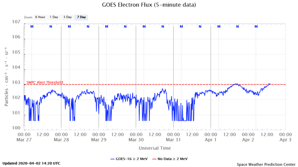
Different SWx centres use different alert and warning thresholds. The alert used by NOAA/SWPC is probably the best known and is issued when the electron flux exceeds 1000 pfu (1 pfu = 1 particle flux unit = 1 electron / cm2 sr s ) for more than three consecutive five-minute periods. This is the red dashed line indicated on their online GOES plot at (see example underneath).
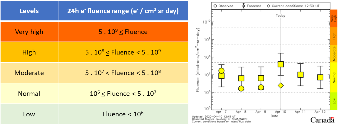
However, the electron flux at geostationary orbit has diurnal variations, with higher fluxes measured near noon and lower fluxes near midnight due to local time asymmetry of Earth’s magnetic field. Therefore, in order to eliminate the local time effects, a daily value of fluence (which is an accumulation over 24h of the electron flux, in units of electrons / cm2 sr day) was used. A qualitative description of the 24 hours electron fluence can be done using the terminology applied by the Canadian SWx centre NRCan. Note fluence values greater than 5 . 107 electrons / cm2 sr day are indicative of adverse space weather conditions hazardous to geosynchronous satellites.
